Chapter 3 Getting and Cleaning Data

3.1 Ch. 3 Objectives

This chapter is designed around the following learning objectives. Upon completing this chapter, you should be able to:

Recognize what a flat file is and how it differs from data stored in a binary file format
Distinguish between delimited and fixed width formats for flat files
Identify the delimiter in a delimited file
Describe a working directory
Demonstrate how to read in different types of flat files
Demonstrate how to read in a few types of binary files (e.g., Matlab, Excel)
Recognize the difference between relative and absolute file pathnames
Describe the basics of your computer’s directory structure
Reference files in your directory structure using relative and absolute pathnames
Apply the basic dplyr functions (e.g., rename(), select(), mutate(), slice(), filter(), and arrange()) to work with data in a dataframe object
Define a logical operator and know the R syntax for common logical operators
Apply logical operators in conjunction with dplyr’s filter() function to create subsets of a dataframe based on logical conditions
Apply a sequence of dplyr functions to a dataframe using piping (%>%)
Create R Markdown documents and describe their basic content and function

3.2 Overview

There are four basic steps you will often repeat as you prepare to analyze data in R:

Identify the location of the data. If it’s on your computer, which directory? If it’s online, what link?
Read data into R (e.g., using a function like read_delim() or read_csv() from the readr package) using the file path you figured out in step 1
Check to make sure the data came in correctly using functions like dim(), head(), tail(), str(), and/or glimpse().
Clean the data up by removing missing (or nonsense) values, renaming or reclassifying variables, performing units conversions, or other actions that support a streamlined data analysis.

In this chapter, I’ll go over the basics for each of these steps and dive a bit deeper into some related topics you should learn now to make your life easier as you get started using R for data analysis.

3.3 Reading data into R

Data comes in files of all shapes and sizes. R has the capability to import data from many files types and locations, even proprietary files for other software. Here are some of the types of data files that R can read and work with:

Flat files (more about these soon)
Files from other software packages such as MATLAB or Excel
Tables on webpages (e.g., the table on Ebola outbreaks near the end of this Wikipedia page)
Data in a database (e.g., MySQL, Oracle)
Data in JSON and XML formats
Really crazy data formats used in other disciplines (e.g., TDMS files from LabView, netCDF files from climate research, MRI data stored in Analyze, NIfTI, and DICOM formats)
Geographic shapefiles
Data through Application Programming Interfaces (APIs; most websites use APIs to ask you for input and then use that input to direct new information back to you)

Often, it is possible to import and wrangle extremely messy data by using functions like scan() and readLines() to read the data in a line at a time, and then using regular expressions to clean up the data as it gets imported. For this course, however, we will begin with less challenging file formats (and degrees of messiness).

3.3.1 Reading local flat files

Much of the data that you will want to read in will be in flat files that are stored locally (i.e., on your computer’s hard drive). A flat file is basically a file that you can open using a text editor. The most common type you’ll work with are probably comma-separated files, often with a .csv or .txt file extension. Most flat files come in two general categories:

Fixed width files, and
Delimited files, which include:

“.csv”: Comma-separated values
“.tab”, “.tsv”: Tab-separated values
Other possible delimiters: colon, semicolon, pipe (“|”)

Fixed-width files are files where a column always has the same width, for all the rows in the column. These tend to look very neat and easy-to-read when you open them in a text editor. For example, the first few rows of a fixed-width file might look like this:

Course                            Number          Day          Time
Thermodynamics                    337             M/W/F        9:00-9:50
Aerosol Physics and Technology    577             M/W/F        10:00-10:50

Fixed-width files used to be very popular, and they make it easier to look at data when you open the file in a text editor. Now, it’s rare to just use a text editor to open a file and check out the data. Also, these files can be a bit of a pain to read into R and other programs because you sometimes have to specify the length of each column. You may come across a fixed-width file every now and then, particularly when working with older data, so it’s useful to be able to recognize one and to know how to import it.

Delimited files use some delimiter such as a comma or tab to separate each column value within a row. The first few rows of a delimited file might look like this:

Course, Number, Day, Time
"Thermodynamics", 337, "M/W/F", "9:00-9:50"
"Aerosol Physics and Technology", 577, "M/W/F", "10:00-10:50"

Delimited files are very easy to read into R. You just need to be able to figure out what character is used as a delimiter and specify that to R in the function call to read in the data.

These flat files can have a number of different file extensions. The most generic is .txt, but they will also have ones more specific to their format, like .csv for a comma-delimited file (.csv stands for “comma-separated values”), or .fwf for a fixed-width file.

R can read in data from both fixed-width and delimited flat files. The only catch is that you need to tell R a bit more about the format of the flat file, including whether it is fixed-width or delimited. If the file is fixed-width, you will usually have to provide R with information about each column (see read_fwf() for details). If the file is delimited, you’ll need to tell R which delimiter, such as comma or tab, is being used.

The read_delim() family of functions are used to read delimited flat files into R - these functions come from the readr package, which we will use extensively in ths course. All members of the read_delim() family do the same basic thing: import flat files into a tibble. The major difference is what defaults each function has for the delimiter (delim). Members of the read_delim() family include:

Function	Delimiter
`read_csv()`	comma
`read_csv2()`	semi-colon
`read_table2()`	whitespace
`read_tsv()`	tab

You can use read_delim() to read in any delimited file, regardless of the delimiter; however, you will need to specify the type of delimiter using the delim argument. If you remember the more specialized function call (e.g., read_csv() for a comma-delimited file), you can save yourself some typing.

For example, to read in the Ebola data data file, which is comma-delimited, you could either use read_table() with a delim argument specified or use read_csv(), in which case you don’t have to specify delim:

library(package = "readr")
# The following two calls do the same thing
ebola <- readr::read_delim(file = "data/country_timeseries.csv", delim = ",")

ebola <- readr::read_csv(file = "data/country_timeseries.csv")

## Rows: 122 Columns: 18
## ── Column specification ────────────────────────────────────────────────────────
## Delimiter: ","
## chr  (1): Date
## dbl (17): Day, Cases_Guinea, Cases_Liberia, Cases_SierraLeone, Cases_Nigeria...
## 
## ℹ Use `spec()` to retrieve the full column specification for this data.
## ℹ Specify the column types or set `show_col_types = FALSE` to quiet this message.

The message that R prints after this call (“Parsed with column specification: …”) lets you know what classes were used for each column. This function tries to guess the appropriate class and typically gets it right. You can suppress the message using the cols_types = cols() argument, or by adjusting the code chunk options in an R Markdown. If readr doesn’t correctly assign some of the columns classes, you can use the type_convert() function for R to guess again after you’ve tweaked the formats of the rogue columns.

This family of functions has a few other helpful options you can specify. For example, if you want to skip the first few lines of a file before you start reading in the data, you can use skip() to set the number of lines to skip. If you only want to read in a few lines of the data, you can use the n_max() option. For example, if you have a really large file, and you want to save time by only reading in the first ten lines, as you figure out what other optional arguments to use in read_delim() for that file, you could include the option n_max = 10. Here is a table of some of the most useful options common to the read_delim() family of functions:

Option	Description
`skip()`	How many lines of the start of the file should you skip?
`col_names()`	Use the column names provided or define your own names?
`col_types()`	What are the column types (e.g., chr, num, int, logi etc.])?
`n_max()`	How many rows do you want to read in?
`na()`	How are missing values coded?

Remember that you can always find out more about a function by looking at its help file. For example, check out ?read_delim and ?read_fwf (note the lack of parentheses). You can also use the help files to determine the default values of arguments for each function.

So far, we’ve only looked at functions from the readr package for reading in data files. There is a similar family of functions available in base R, the read.table() family of functions. The readr family of functions is very similar to the base R read.table() functions, but have some more sensible defaults. Compared to the read.table() function family, the readr functions are:

Faster; show progress bar of data import
Work better with large datasets
Have more sensible defaults (e.g., characters default to characters, not factors)

I recommend that you always use the readr functions rather than their base R alternatives, given these advantages; however, you are likely to come across code with these base R functions, so it is helpful to be aware of them. Functions in the read.table family include:

read.csv()
read.delim()
read.table()
read.fwf()

Note: these base R functions use periods (read.) whereas the readr functions use underscores (read_).

The readr package is a member of the tidyverse suite of R packages. The tidyverse describes an evolving collection of R packages with a common philosophy and approach, and they are unquestionably changing the way people code in R. Many of these R packages were developed in part or full by Hadley Wickham and others at RStudio. Many of these packages are less than ten years old but have been rapidly adapted by the R community. As a result, newer examples of R code will often look very different from the code in older R scripts, including examples in books that are more than a few years old. In this course, I’ll focus on tidyverse functions when possible, but I do put in details about base R equivalent functions or processes at some points. This will help you interpret older code. You can download all the tidyverse packages at the same time with install.packages(“tidyverse”) and make all the tidyverse functions available for use withlibrary(“tidyverse”).

3.3.2 Reading in other file types

Later in the course, we’ll talk about how to open a variety of other file types in R. You might find it immediately useful to be able to read in files from other statistical programs.

There are two “tidyverse” packages, readxl and haven, that help with this. They allow you to read in files from the following formats:

File type	Function	Package
Excel	`read_excel()`	`readxl`
SAS	`read_sas()`	`haven`
SPSS	`read_spss()`	`haven`
Stata	`read_stata()`	`haven`

3.4 Directories and pathnames

3.4.1 Directory structure

So far, we’ve only looked at reading in files that are located in your current working directory. For example, if you’re working in an R Project, by default the project will open with that directory as the working directory, so you can read files that are saved in that project’s main directory using only the file name as a reference.

You will often want to read in files that are located somewhere else on your computer, or even files that are saved on another computer or posted online. Doing this is very similar to reading in a file that is in your current working directory; the only difference is that you need to give R some directions so it can find the file.

The most common case will be reading in files in a subdirectory of your current working directory. For example, you may have created a “data” subdirectory in one of your R Projects directories to keep all the project’s data files in the same place while keeping the structure of the main directory fairly clean. In this case, you’ll need to direct R into that subdirectory when you want to read one of those files.

To understand how to give R these directions, you need to have some understanding of the directory structure of your computer. It seems a bit of a pain and a bit complex to have to think about computer directory structure in the “basics” part of this class, but this structure is not terribly complex once you get the idea of it. There are a couple of very good reasons why it’s worth learning now.

First, many of the most frustrating errors you get when you start using R trace back to understanding directories and filepaths. For example, when you try to read a file into R using only the filename, and that file is not in your current working directory, you will get an error like:

Error in file(file, "rt") : cannot open the connection
In addition: Warning message:
In file(file, "rt") : cannot open file 'Ex.csv': No such file or directory

This error is especially frustrating when you’re new to R because it happens at the very beginning of your analysis—you can’t even import the data. Also, if you don’t understand a bit about working directories and how R looks for the file you’re asking it to find, you’d have no idea where to start to fix this error. Second, once you understand how to use pathnames, especially relative pathnames, to tell R how to find a file that is in a directory other than your working directory, you will be able to organize all of your files for a project in a much cleaner way. For example, you can create a directory for your project, then create one subdirectory to store all of your R scripts, and another to store all of your data, and so on. This can help you keep very complex projects more structured and easier to navigate.

Your computer organizes files through a collection of directories. Chances are, you are fairly used to working with these in your daily life already, although you may call them “folders” rather than “directories”. For example, you’ve probably created new directories to store data files and Word documents for a specific project.

Figure 3.1 gives an example file directory structure for a hypothetical computer. Directories are shown in blue, and files in green.

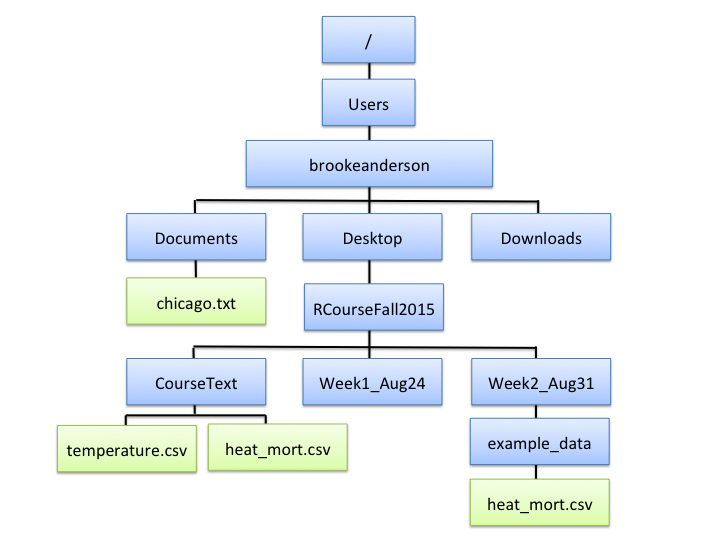
Figure 3.1: An example of file directory structure.

Notice a few interesting things from Figure 3.1. First, you might notice the structure includes a few of the directories that you use a lot on your own computer, like Desktop, Documents, and Downloads. Next, the directory at the very top is the computer’s root directory, /. For a PC, the root directory might something like C:. For Unix and Macs, it’s usually /. Finally, if you look closely, you’ll notice that it’s possible to have different files in different locations of the directory structure with the same file name. For example, in the figure, there are files names heat_mort.csv in both the CourseText directory and in the example_data directory. These are two different files with different contents, but they can have the same name as long as they’re in different directories. This fact—that you can have files with the same name in different places—should help you appreciate how useful it is that R requires you to give very clear directions to describe exactly which file you want R to read in, if you aren’t importing something in your current working directory.

You will have a home directory somewhere near the top of your structure, although it’s likely not your root directory. In the hypothetical computer in Figure 3.1, the home directory is /Users/brookeanderson. I’ll describe just a bit later how you can figure out what your own home directory is on your own computer.

3.4.2 Working directory

When you run R, it’s always running from within some working directory, which will be one of the directories somewhere in your computer’s directory structure. At any time, you can figure out which directory R is working in by running the command getwd() (short for “get working directory”). For example, my R session is currently running in the following directory:

getwd()

## [1] "/Users/johnvolckens/Teaching/DataSci/edar_coursebook"

This means that, for my current R session, R is working in the edar_coursebook subdirectory of my johnvolckens directory (home directory).

There are a few general rules for which working directory R selects when you open an R session. These are not absolute rules, but they’re generally true. If you have R closed, and you open it by double-clicking on an R script, then R will generally open with, as its working directory, the directory in which that script is stored. This is often a very convenient convention, because often any of the data you’ll import for that script is somewhere near where the script file is saved in the directory structure. If you open R by double-clicking on the R icon in “Applications” (or the start menu on a PC), R will start in its default working directory. You can find out what this is, or change it, in RStudio’s “Preferences”. Finally, if you open an R Project, R will start in that project’s working directory—where the .Rproj file for the project is stored. This is one of the reasons why we always create a new R Project when starting a data analysis - RStudio projects remember where to look!

3.4.3 File and directory pathnames

Once you get a picture of how your directories and files are organized, you can use pathnames, either absolute or relative, to read in files from different directories outside your current working directory. Pathnames are the directions for getting to a directory or file stored on your computer.

When you want to reference a directory or file, you can use one of two types of pathnames:

Relative pathname: How to get to the file or directory from your current working directory
Absolute pathname: How to get to the file or directory from anywhere on the computer

Absolute pathnames are a bit more straightforward conceptually because they don’t depend on your current working directory; however, they’re also a lot longer to write and very inconvenient if you’ll be sharing some of your code with other people who might try to run it on their own computers. I’ll explain this second point a bit more later in this section.

I strongly advise against the use of absolute pathnames because of the aforementioned collaborative issue, but I will include some details here nonetheless. Absolute pathnames give the full directions to a directory or file, starting all the way at the root directory. For example, the daily_show_guests.csv file in the data directory has the absolute pathname:

"/Users/johnvolckens/Teaching/DataSci/edar_coursebook/data/daily_show_guests.csv"

You can use this absolute pathname to read this file in using any of the readr functions to read in data. This absolute pathname will always work, regardless of your current working directory, because it gives directions from the root. In other words, it will always be clear to R exactly what file you’re talking about. Here’s the code to use to read that file in using the read.csv() function with the file’s absolute pathname:

daily_show <- readr::read_csv(file = "/Users/johnvolckens/Teaching/DataSci/edar_coursebook/data/daily_show_guests.csv", skip = 4)

The relative pathname, on the other hand, gives R the directions for how to get to a directory or file from the current working directory. If the file or directory you’re looking for is pretty close to your current working directory in your directory structure, then a relative pathname can be a much shorter way to tell R how to get to the file than an absolute pathname. But, the relative pathname depends on your current working directory—the relative pathname that works perfectly when you’re working in one directory will not work at all once you move into a different working directory.

As an example of a relative pathname, say you’re working directory is edar_coursebook and you want to read in the daily_show_guests.csv file in the data directory (one of the edar_coursebook subdirectories). To get from edar_coursebook to that file, you’d need to look in the subdirectory data, where you could find daily_show_guests.csv. Therefore, the relative pathname from your working directory would be:

"data/daily_show_guests.csv"

You can use this relative pathname to tell R where to find and read in the file:

daily_show <- readr::read_csv("data/daily_show_guests.csv")

While this pathname is much shorter than the absolute pathname, it is important to remember that if you are working in a different working directory, this relative pathname would no longer work.

There are a few abbreviations that can be really useful for pathnames:

Shorthand	Meaning
`~`	Home directory
`.`	Current working directory
`..`	One directory up from current working directory
`../..`	Two directories up from current working directory

These can help you keep pathnames shorter and also help you move “up-and-over” to get to a file or directory that’s not on the direct path below your current working directory.

For example, my home directory is /Users/johnvolckens. You can use the list.files() function to list all the files in a directory. If I wanted to list all the files in my Downloads directory, which is a direct sub-directory of my home directory, I could use:

list.files("~/Downloads")

As a second example, say I was working in the working directory CourseText, (see Figure 3.1 but I wanted to read in the heat_mort.csv file that’s in the example_data directory, rather than the one in the CourseText directory. I can use the .. abbreviation to tell R to look up one directory from the current working directory, and then down within a subdirectory of that. The relative pathname in this case is:

"../Week2_Aug31/example_data/heat_mort.csv"

The ../ tells R to look one directory up from the working directory (the directory that is one level above the current directory is also known as the parent directory), which in this case is to RCourseFall2015, and then down within that directory to Week2_Aug31, then to example_data, and then to look within that directory for the file heat_mort.csv.

The relative pathname to read this file while R is working in the CourseTest directory would be:

heat_mort <- read_csv("../Week2_Aug31/example_data/heat_mort.csv")

Relative pathnames “break” as soon as you try them from a different working directory—this fact might make it seem like you would never want to use relative pathnames, and would always want to use absolute ones instead, even if they’re longer. If that were the only consideration (length of the pathname), then perhaps that would be true. However, as you do more and more in R, there will likely be many occasions when you want to use relative pathnames instead. They are particularly useful if you ever want to share a whole directory, with all subdirectories, with a collaborator. In that case, if you’ve used relative pathnames, all the code should work fine for the person you share with, even though they’re running it on their own computer. Conversely, if you’d used absolute pathnames, none of them would work on another computer, because the “top” of the directory structure (i.e., for me, /Users/johnvolckens/) will definitely be different for your collaborator’s computer than it is for yours.

If you’re getting errors reading in files, and you think it’s related to the relative pathname you’re using, it’s often helpful to use list.files() to make sure the file you’re trying to load is in the directory guided by the relative pathname. The list.files() function is very useful because it returnsa character vector of filenames (and paths, if desired). Once you have a vector of filenames you can do things like ask logical questions (does this file exist?), or count the number of files, or pass a relative path to a new function…

3.4.4 Tangent: `paste`

This is a good opportunity to explain how to use some functions that can be very helpful when you’re using relative or absolute pathnames: paste() and paste0(). It’s important that you understand that you can save a pathname (absolute or relative) as an R object and then use that R object in calls to later functions like list.files() and read_csv(). For example, to use the absolute pathname to read the heat_mort.csv file in the CourseText directory, you could run:

my_file <- "/Users/brookeanderson/Desktop/RCourseFall2015/CourseText/heat_mort.csv"
heat_mort <- read_csv(file = my_file)

You’ll notice from this code that the pathname to get to a directory or file can sometimes become ungainly and long. To keep your code cleaner, you can address this by using the paste or paste0 functions. These functions come in handy in a lot of other applications, too, but this is a good place to introduce them.

The paste() function is very straightforward. It takes, as inputs, a series of different character strings you want to join together, and it pastes them together in a single character string. (As a note, this means that your resulting vector will only be one element long for basic uses of paste(), while the inputs will be several different character stings.) You separate all the different things you want to paste together using with commas in the function call. For example:

paste("Sunday", "Monday", "Tuesday")

## [1] "Sunday Monday Tuesday"

length(x = c("Sunday", "Monday", "Tuesday"))

## [1] 3

length(x = paste("Sunday", "Monday", "Tuesday"))

## [1] 1

The paste() function has an option called sep =. This tells R what you want to use to separate the values you’re pasting together in the output. The default is for R to use a space, as shown in the example above. To change the separator, you can change this option, and you can put in just about anything you want. For example, if you wanted to paste all the values together without spaces, you could use sep = "":

paste("Sunday", "Monday", "Tuesday", sep = "")

## [1] "SundayMondayTuesday"

As a shortcut, instead of using the sep = "" option, you could achieve the same thing using the paste0 function. This function is almost exactly like paste, but it defaults to "" (i.e., no space) as the separator between values by default:

paste0("Sunday", "Monday", "Tuesday")

## [1] "SundayMondayTuesday"

With pathnames, you will usually not want spaces. Therefore, you could think about using paste0() to write an object with the pathname you want to ultimately use in commands like list.files() and setwd(). This will allow you to keep your code cleaner, since you can now divide long pathnames over multiple lines:

my_file <- paste0("/Users/brookeanderson/Desktop/",
                  "RCourseFall2015/CourseText/heat_mort.csv")
heat_mort <- read_csv(file = my_file)

You will end up using paste() and paste0() for many other applications, but this is a good example of how you can start using these functions to start to get a feel for them.

3.4.5 Reading online flat files

So far, I’ve only shown you how to import data from files that are saved to your computer. R can also read in data directly from the web. If a flat file is posted online, you can read it into R in almost exactly the same way that you would read in a local file. The only difference is that you will use the file’s URL instead of a local file path for the file argument.

With the read_* family of functions, you can do this both for flat files from a non-secure webpage (i.e., one that starts with http) and for files from a secure webpage (i.e., one that starts with https), including GitHub and Dropbox.

For example, to read in data from this GitHub repository of Ebola data, you can run:

url <- paste0("https://raw.githubusercontent.com/cmrivers/",
              "ebola/master/country_timeseries.csv")
ebola <- readr::read_csv(file = url)
slice(.data = (dplyr::select(.data = ebola, 1:3)), 1:3)

## # A tibble: 3 × 3
##   Date       Day Cases_Guinea
##   <chr>    <dbl>        <dbl>
## 1 1/5/2015   289         2776
## 2 1/4/2015   288         2775
## 3 1/3/2015   287         2769

3.5 Data cleaning

Once you have loaded data into R, you’ll likely need to clean it up a little before you’re ready to analyze it. Here, I’ll go over the first steps of how to do that with functions from dplyr, another package in the tidyverse. Here are some of the most common data-cleaning tasks, along with the corresponding dplyr function for each:

Task	`dplyr` function
Renaming columns	`rename()`
Filtering to certain rows	`filter()`
Selecting certain columns	`select()`
Adding or changing columns	`mutate()`

In this section, I describe how to do each of these four tasks. For the examples in this section, I use example data listing guests to the Daily Show. To follow along with these examples, you’ll want to load that data, as well as load the dplyr package. Install it using install.packages() if you have not done so already.

library("dplyr")
daily_show <- readr::read_csv(file = "data/daily_show_guests.csv", skip = 4)

I’ve used this data in previous examples, but as a reminder, here’s what it looks like:

head(x = daily_show)

## # A tibble: 6 × 5
##    YEAR GoogleKnowlege_Occupation Show    Group  Raw_Guest_List  
##   <dbl> <chr>                     <chr>   <chr>  <chr>           
## 1  1999 actor                     1/11/99 Acting Michael J. Fox  
## 2  1999 Comedian                  1/12/99 Comedy Sandra Bernhard 
## 3  1999 television actress        1/13/99 Acting Tracey Ullman   
## 4  1999 film actress              1/14/99 Acting Gillian Anderson
## 5  1999 actor                     1/18/99 Acting David Alan Grier
## 6  1999 actor                     1/19/99 Acting William Baldwin

3.5.1 Renaming columns

A first step is often renaming the columns of the dataframe. It can be hard to work with a column name that:

is long
includes spaces or other special characters
includes uppercase letters

You can check out the column names for a dataframe using the colnames() function, with the dataframe object as the argument. Several of the column names in daily_show have some of these issues:

colnames(x = daily_show)

## [1] "YEAR"                      "GoogleKnowlege_Occupation"
## [3] "Show"                      "Group"                    
## [5] "Raw_Guest_List"

To rename these columns, use rename(). The basic syntax is:

## generic code; will not run
dplyr::rename(.data = dataframe,
              new_column_name_1 = old_column_name_1,
              new_column_name_2 = old_column_name_2)

The first argument is the dataframe for which you’d like to rename columns. Then you list each pair of new and old column names (in that order) for each of the columns you want to rename. To rename columns in the daily_show data using rename(), for example, you would run:

daily_show <- dplyr::rename(.data = daily_show,
                            year = YEAR,
                            job = GoogleKnowlege_Occupation,
                            date = Show,
                            category = Group,
                            guest_name = Raw_Guest_List)
head(x = daily_show, 3)

## # A tibble: 3 × 5
##    year job                date    category guest_name     
##   <dbl> <chr>              <chr>   <chr>    <chr>          
## 1  1999 actor              1/11/99 Acting   Michael J. Fox 
## 2  1999 Comedian           1/12/99 Comedy   Sandra Bernhard
## 3  1999 television actress 1/13/99 Acting   Tracey Ullman

Many of the functions in tidyverse packages, including those in dplyr, provide exceptions to the general rule about quotation marks. Unfortunately, this may make it a bit hard to learn when to use quotation marks. One way to think about this, which is a bit of an oversimplification but can help as you’re learning, is to assume that anytime you’re using a dplyr function, every column in the dataframe you’re working with has been loaded to your R session as its own object, which means you don’t need to use parentheses—most of the time.

If you have been paying close attention to the code snippets, you may have noticed the last bit of code included both the package name and the function call separated by two colons, as in dplyr::rename(). This syntax of package.name::package.function is used for the sake of being explicit, because (as you may have guessed) some R packages use the same for functions that do entirely different things! For example, both the base R stats package and the dplyr package have a function called filter() - the former is used to pick our rows from a data frame and the latter is used to manipulate time-series objects. When two packages are loaded containing functions with the same name, R will default to using the function for the most recently loaded package (and send you a message stating as much). This can be tricky business when your R session has many packages running, which is why it never hurts to be explicit in your function calls.

3.5.2 Selecting columns

Next, you may want to select only some columns of the dataframe. You can use the select() function from dplyr to subset the dataframe to certain columns. The basic structure of this command is:

## generic code; will not run
dplyr::select(.data = dataframe, column_name_1, column_name_2, ...)

In this call, you first specify the dataframe to use and then list all of the column names to include in the output dataframe, with commas between each column name. For example, to select all columns in daily_show except year (since that information is already included in date), run:

dplyr::select(.data = daily_show, job, date, category, guest_name)

## # A tibble: 2,693 × 4
##    job                date    category guest_name      
##    <chr>              <chr>   <chr>    <chr>           
##  1 actor              1/11/99 Acting   Michael J. Fox  
##  2 Comedian           1/12/99 Comedy   Sandra Bernhard 
##  3 television actress 1/13/99 Acting   Tracey Ullman   
##  4 film actress       1/14/99 Acting   Gillian Anderson
##  5 actor              1/18/99 Acting   David Alan Grier
##  6 actor              1/19/99 Acting   William Baldwin 
##  7 Singer-lyricist    1/20/99 Musician Michael Stipe   
##  8 model              1/21/99 Media    Carmen Electra  
##  9 actor              1/25/99 Acting   Matthew Lillard 
## 10 stand-up comedian  1/26/99 Comedy   David Cross     
## # ℹ 2,683 more rows

Don’t forget that, if you want to change column names in the saved object, you must reassign the object to be the output of rename(). If you run one of these cleaning functions without reassigning the object, R will print out the result, but the object itself won’t change. You can take advantage of this, as I’ve done in this example, to look at the result of applying a function to a dataframe without changing the original dataframe. This can be helpful as you’re figuring out how to write your code.

The select() function also provides some time-saving tools. In the last example, we wanted all the columns except one. Instead of writing out all the columns we want, we can use - with only the columns we don’t want to save time (notice the object reassignment/override):

daily_show <- dplyr::select(.data = daily_show, -year)
head(x = daily_show, n = 3)

## # A tibble: 3 × 4
##   job                date    category guest_name     
##   <chr>              <chr>   <chr>    <chr>          
## 1 actor              1/11/99 Acting   Michael J. Fox 
## 2 Comedian           1/12/99 Comedy   Sandra Bernhard
## 3 television actress 1/13/99 Acting   Tracey Ullman

3.5.3 Add or change columns

You can change a column or add a new column using the mutate() function from the dplyr package. That function has the syntax:

# generic code; will not run
dplyr::mutate(.data = dataframe,
              changed_column = function(changed_column),
              new_column = function(other arguments))

For example, the job column in daily_show sometimes uses upper case and sometimes does not. This call uses the unique() function to list only unique values in this column:

head(x = unique(x = daily_show$job), n = 10)

##  [1] "actor"              "Comedian"           "television actress"
##  [4] "film actress"       "Singer-lyricist"    "model"             
##  [7] "stand-up comedian"  "actress"            "comedian"          
## [10] "Singer-songwriter"

To make all the observations in the job column lowercase, use the str_to_lower() function from the stringr package within a mutate() function:

library(package = "stringr")
mutate(.data = daily_show, 
       job = str_to_lower(string = job))

## # A tibble: 2,693 × 4
##    job                date    category guest_name      
##    <chr>              <chr>   <chr>    <chr>           
##  1 actor              1/11/99 Acting   Michael J. Fox  
##  2 comedian           1/12/99 Comedy   Sandra Bernhard 
##  3 television actress 1/13/99 Acting   Tracey Ullman   
##  4 film actress       1/14/99 Acting   Gillian Anderson
##  5 actor              1/18/99 Acting   David Alan Grier
##  6 actor              1/19/99 Acting   William Baldwin 
##  7 singer-lyricist    1/20/99 Musician Michael Stipe   
##  8 model              1/21/99 Media    Carmen Electra  
##  9 actor              1/25/99 Acting   Matthew Lillard 
## 10 stand-up comedian  1/26/99 Comedy   David Cross     
## # ℹ 2,683 more rows

We will take a deeper dive into strings and the stringr package later on.

3.5.4 Base R equivalents to `dplyr` functions

Just so you know, all of these dplyr functions have alternatives, either functions or processes, in base R:

`dplyr`	Base R equivalent
`rename()`	Reassign `colnames()`
`select()`	Square bracket indexing
`filter()`	`subset()`
`mutate()`	Use `$` to change or create columns
`slice()`	`subset()` with logical expression

You will see these alternatives used in older code examples. Some of these functions have variants specific to particular data wrangling needs. For example, under slice(), there are others such as slice_max() and slice_min(), which extract the top and bottom values, respectively, from a dataset based on user input in the required arguments, including n and order_by.

3.5.5 Filtering to certain rows

Next, you might want to filter the dataset to certain rows. For example, you might want to get a dataset with only the guests from 2015, or only guests who are scientists.

You can use the filter() function from dplyr to filter a dataframe down to a subset of rows. The syntax is:

## generic code; will not run
filter(.data = dataframe, logical expression)

The logical expression in this call gives the condition that a row must meet to be included in the output data frame. For example, if you want to create a data frame that only includes guests who were scientists, you can run:

scientists <- filter(.data = daily_show, 
                     category == "Science")
head(x = scientists)

## # A tibble: 6 × 4
##   job            date    category guest_name            
##   <chr>          <chr>   <chr>    <chr>                 
## 1 neurosurgeon   4/28/03 Science  Dr Sanjay Gupta       
## 2 scientist      1/13/04 Science  Catherine Weitz       
## 3 physician      6/15/04 Science  Hassan Ibrahim        
## 4 doctor         9/6/05  Science  Dr. Marc Siegel       
## 5 astronaut      2/13/06 Science  Astronaut Mike Mullane
## 6 Astrophysicist 1/30/07 Science  Neil deGrasse Tyson

To build a logical expression to use in filter, you’ll need to know some of R’s logical operators. Some commonly used ones are:

Operator	Meaning	Example
`==`	equals	`category == "Acting"`
`!=`	does not equal	`category != "Comedy`
`%in%`	match; contains the following	`category %in% c("Academic", "Science")`
`is.na()`	is missing	`is.na(job)`
`!is.na()`	is not missing	`!is.na(job)`
`&`	and	`year == 2015 & category == "Academic"`
`\|`	or	`year == 2015 \| category == "Academic"`

We’ll use these logical operators and expressions a lot more as the course continues, so they’re worth memorizing.

Two common mistakes with logical operators are: (1) Using = instead of == to check if two values are equal; and (2) Using == NA instead of is.na to check for missing observations.

3.6 Merging Data Frames

Many data analysis exercises will require you to combine data from different sources into a single object. Thus, it’s worthwhile to understand how R can be used to merge together two or more data frames.

Merging data frames is generally done in one of two ways, depending on how those data frames are similar: row binding or column binding. Below, I provide reference to dplyr:: functions, but, as usual, there are base R functions (rbind() and cbind()) that work, too!

3.6.1 Row Binding

Row binding can be performed whenever the two (or more) data frames have column variables in common. Figure 3.2 shows this process graphically. Since the x and y data frames have identical column variables, the rows of data (i.e., what’s under the column names) can be “staked” on top of each other to create a single data frame.

This is accomplished in the example using dplyr::bind_rows(x, y).

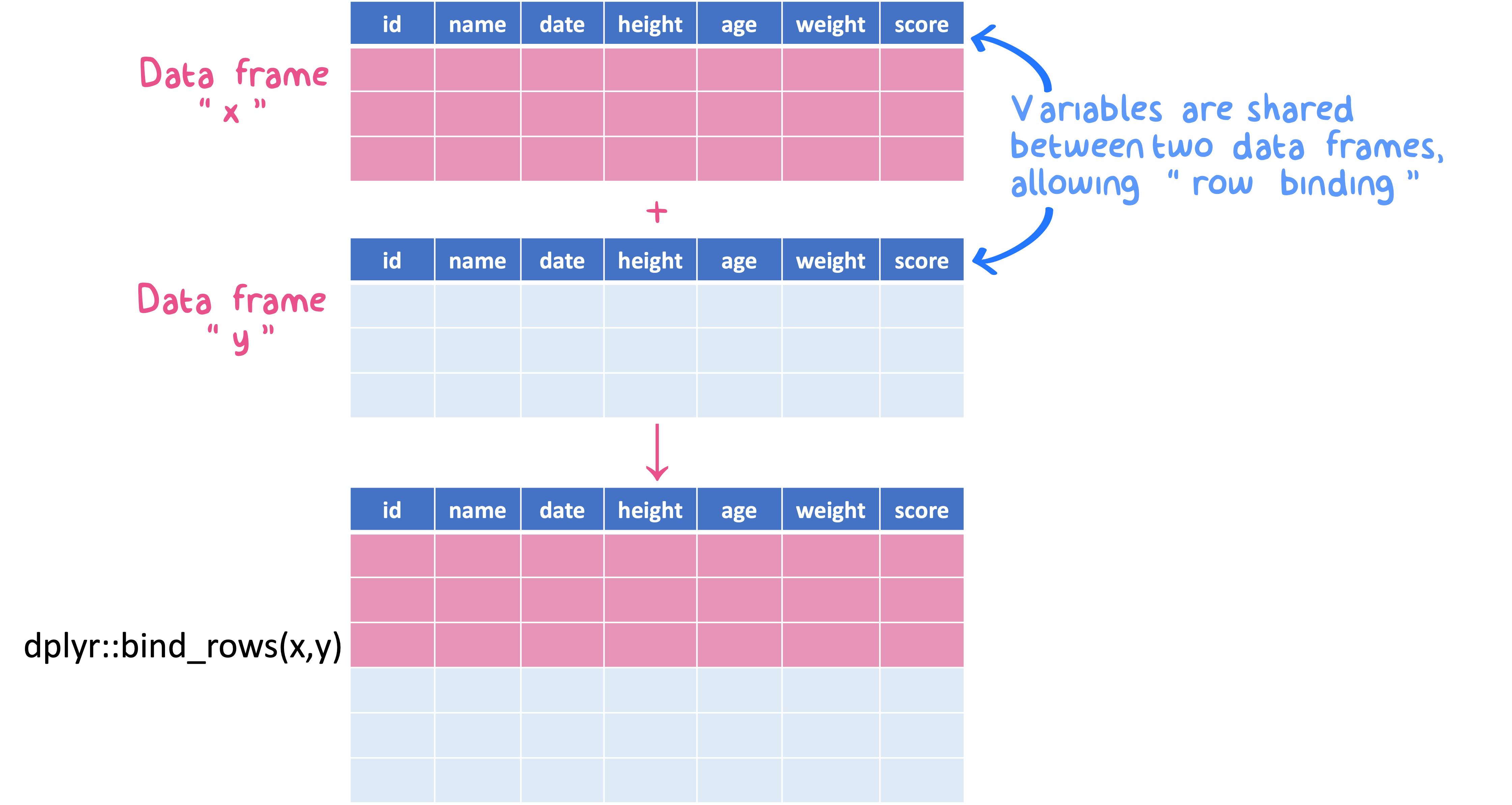
Figure 3.2: Row binding can occur when data frames x and y share the column variables.

Note that if the x and y data frames have column variables that are not shared, those variables will be carried forward but the observations will contain NA. Therefore, you should always check your resultant data frame for completeness using functions like complete.cases() or a combination of is.na() with sum() or which().

3.6.2 Column Binding (_join)

Data frames can also be merged when row observations are shared, such that you end up merging column variables together from two objects. In this case, we would join the two data frames using a function like dplyr::left_join(). To do this, we must specify one or more variables that can uniquely identify row observations that are common between the two data frames. Once the rows are “lined up”, we can paste the new column variables into a combined data frame. This is shown schematically in Figure 3.3 where the matching rows are specified using the argument by = var_a within the join function.

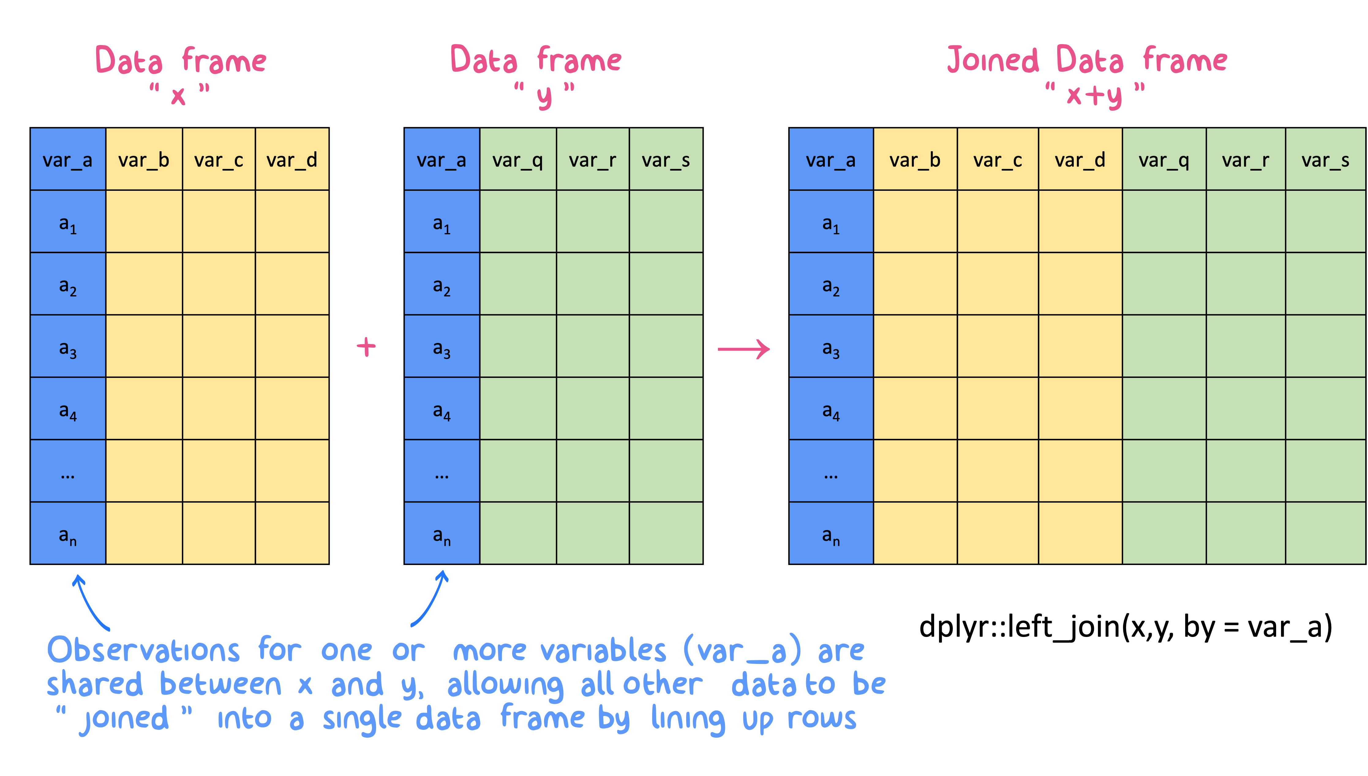
# generic code for example; will not run
new.dataframe <- left_join(x, y, by = var_a)

Figure 3.3: Column binding, or joins can occur when data frames x and y share the same row observations.

The dplyr:: package features a number of mutate-join functions (e.g., left_join(), right_join(), inner_join()) that add columns from data frame y to data frame x, once you specify how to match rows using the by = argument.

inner_join(): includes all rows in x and y (regardless of whether they match).
left_join(): includes all rows in x (and only y rows if they match).
right_join(): includes all rows in y.
full_join(): includes all rows in x or y.

Note that if your matching key (by =) does not produce unique row observations (for example, if you had two different "John" entries in a variable called first.name between both data frames) then R will create duplicate row entries that account for the possible combinations of the John observation in x with the John observation in y. One way to check for this is to look at the length() of the resultant (merged) data frame. In most cases, it should have the same length as the starting data frame, contingent on which mutate-join function you call. Another way is to look for duplicate observations in the data frame using the inverse unique()function on your key variable !unique() or the duplicated() function.

3.7 Piping

So far, I’ve shown how to use these dplyr functions one at a time to clean up the data, reassigning the dataframe object at each step; however, there’s a trick called “piping” (with %>%) that will let you complete multiple data wrangling steps at once.

If you look at the format of these dplyr functions, you’ll notice that they all take a dataframe as their first argument:

# generic code; will not run
rename(.data = dataframe, 
       new_column_name_1 = old_column_name_1,
       new_column_name_2 = old_column_name_2)
select(.data = dataframe, 
       column_name_1, column_name_2)
filter(.data = dataframe, 
       logical expression)
mutate(.data = dataframe,
       changed_column = function(changed_column),
       new_column = function(other arguments))

Without piping, you have to reassign the dataframe object at each step of this cleaning if you want the changes saved in the object:

daily_show <-read_csv(file = "data/daily_show_guests.csv",
                      skip = 4)
daily_show <- rename(.data = daily_show, 
                     job = GoogleKnowlege_Occupation,
                     date = Show,
                     category = Group,
                     guest_name = Raw_Guest_List)
daily_show <- select(.data = daily_show, 
                     -YEAR) 
daily_show <- mutate(.data = daily_show, 
                     job = str_to_lower(job))
daily_show <- filter(.data = daily_show, 
                     category == "Science")

Piping lets you streamline this process. It can be used with any function that inputs a dataframe (or vector) as its first argument. The %>% operator pipes the object on the left-hand-side of the pipe (%>%) into the function on the right-hand-side (immediately after the pipe). With piping, therefore, all of the data cleaning steps shown avove would look like:

daily_show <- readr::read_csv(file = "data/daily_show_guests.csv",
                              skip = 4) %>%
  dplyr::rename(job = GoogleKnowlege_Occupation,
                date = Show,
                category = Group,
                guest_name = Raw_Guest_List) %>%
  dplyr::select(-YEAR) %>%
  dplyr::mutate(job = str_to_lower(job)) %>%
  dplyr::filter(category == "Science")

Notice that, when piping a data frame, the first argument (name of the data frame) is excluded from all function calls that follow a pipe. This is because piping sends the dataframe from the last step into each of the following functions as the dataframe argument. Remember: Order matters in a data wrangling pipeline. For example, if you remove a column in an early line of code in the pipeline but then reference that column name later, R will throw an error. You can use selective highlighting to run one line at a time to see how the dataframe changes in real-time as you move through successive pipes.

Piping with %>% should only be used when you want to perform succesive data wrangling steps on a single object. Each pipe operation should be followed by a new line, as shown above. Creating a new line after each pipe step aids readability of the pipe, since each new action occurs on a new line of code. Also, if a single pipe function contains multiple arguments, consider putting each argument on a separate line, too (also shown in the code snippet above).

3.8 Markdowns

A markdown is a file format designed for the internet. Markdown files allow you to enter plain text into a file, format that text, and embed code/images/data into the file (everything you are reading in this coursebook was written and created with markdown files).
Markdown files are versatile because:

Markdowns can be rendered into html, pdf, and doc files easily. Thus, markdown files can be turned into websites, email messages, reports, blogs, textbooks, and other forms of media without worry;
Markdowns are independent of the operating system (Mac, PC, Linux, Android, and iOS devices can read them);
Markdowns can be opened by almost any application (the file format is non-proprietary), so you don’t need to worry about having special software to read them.
A markdown document provides an excellent template for reproducible research - allowing you to communicate what you did, how and why you did it, what you found, and any conclusions (or follow-on questions) you can draw from the work.

3.8.1 R Markdowns

The R Studio IDE can create “R Markdowns” (file extension .Rmd) specifically for the R programming environment. An R markdown file allows you do lots of things; we will use them to create assignments and homework reports that display R code, the outputs of that code, and plain text. To use the R markdown format, you need to install the rmarkdown package: install.packages("rmarkdown").

Going forward, all of your homework and coding assignments will be created and submitted in the R Markdown format using either html or pdf outputs. This may seem uncomfortable at first but you will get accustomed to this format quickly.

Each R markdown file contains three basic elements: header, text, and code chunks. I will explain each of these elements below, but I recommend a visit to the R Markdown section on the RStudio website. A detailed guide on many of the R markdown output styles (beyond just html and pdf files) is provided in R Markdown: The Definitive Guide.

3.8.2 Header

The R Markdown “header” section is where you specify details about the file being created. A markdown header contains YAML metadata, which stands for “YAML Ain’t Markup Language”. The YAML (pronounced like “camel”) header is essentially a list of directives (referred to as “key:value” pairs) that help application software interpret the file. A YAML header can act simultaneously as a “configuration file”, a “log file”, and “translator file” - allowing one software program to read the output of another program. An example header with YAML metadata is shown below.

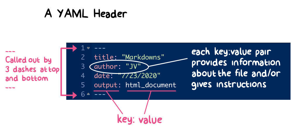
Figure 3.4: Example of a YAML header to render an R Markdown into an html file.

The header is delineated at the top of the file by a section that begins and ends with three dashes, “—”. Within the header are YAML metadata representing key:value pairs. What are “key:value” pairs? The “key:” is a directive that you want to give to the file and the “value” represents the level of detail or information that you want to associate with that directive. Key:value pairs provide instructions on how the file should be read, interpreted, and output. In Figure 3.4, the keys are “title:”, “author:”, “date:”, and “output:” and the corresponding values are “Markdowns”, “JV”, “7/23/2020”, and “html_document”. You can learn more about key:value pairs in the R Markdown Style Guide for html and pdf.

The YAML header is optional in an R Markdown and default key:value pairs will be implemented if none are supplied. That said, I would encourage you to specify key directives like “author:”, “date:” and “output:” in your YAML headers.

Sometimes, you will want to provide nested formatting directives in your markdown header. For example, you can specify the addition of a “table of contents” to your html output file that “floats” alongside the text. In that case, your YAML metadata would look like this:

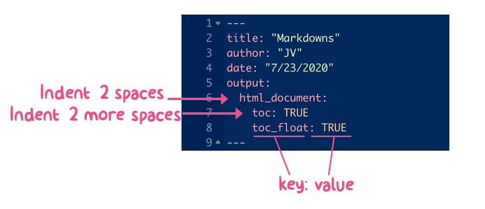
Figure 3.5: Example R Markdown header with nested YAML directives to render an html file with a floating table of contents.

An important detail to remember with nested YAML metadata is that each nested command must be indented by 2 spaces to be interpreted properly.

3.8.3 Text

The default space within an R markdown is a plain text editor, similar to a normal word processing file. Formatting text is more tedious in markdown files (a small price to pay given their versatility). Some basic formatting operations are shown below.

Format Desired	Typeset in Markdown	Example Output
Italics	one star on each side	one star on each side
Bold	two stars on each side	two stars on each side
Superscript	superscript^2^	superscript²
Subscript	subscript~2~	subscript₂

To start a new paragraph in a markdown text section, end a line with two spaces (followed by a return).

To see a more complete set of formatting options see the R Markdown CheatSheet provided by RStudio.

3.8.4 Code Chunks

Code chunks are the places where you write and execute R code. A code chunk is initiated with 3 back ticks ```, followed by a set of braces { }, or curly brackets, within which you can name the chunk and specify chunk options. The chunk options tell the knitr package (the package that renders an R markdown into an output style) how you want that chunk to run and what to do with the output. A list of chunk options can be found here. An example markdown is shown below:

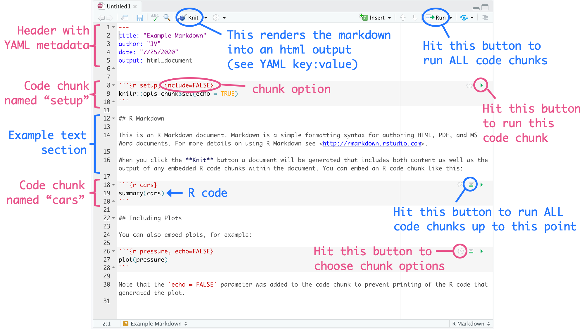
Figure 3.6: Example R Markdown showing header, text, and code chunks.

Once your markdown is complete, you can render it into an output file (e.g., html, pdf, doc, rtf) using the knitr package, which interprets your YAML header and “knits” the markdown sections into the desired format. Here is the same markdown rendered into an html document using the knit button.

Figure 3.7: Example R Markdown when “rendered” into an html document.

3.9 Chapter 3 Exercises

The following sections includes exercises for each lecture regarding Chapter 3. Rhetorical or group discussion questions are also included to help you think about why we are making certain workflow recommendations and to get you in the habit of doing these things regularly. Throughout, I included challenge questions will require you to look outside of the lecture and coursebook. These are optional and do not include answers within the coursebook, but give them a shot. They cover concepts that are important to you as an independent R programmer.

3.9.1 Set 1: Pathnames and data import

Open your class R Project locally. Restart session, if your R Project is already open. Create an R script (e.g., ch-3-exercises.R) and save it in the /code folder.
In the RStudio Console, determine your current working directory. Make sure the working directory is pointed to the location of ch-3-exercises.R within your R Project. If it is not, navigate to Session > Set Working Directory > To Source File Location. Again, check your current working directory to confirm.
Write “metadata” at the top of the R script using #, including your name, today’s date, class, and chapter. Add a heading called “Pathnames and Data Import”.
Download the Fort Collins ozone dataset locally and save the .csv file in the /data folder in your R Project. What would be a better, more descriptive name for the data file that also follows file-naming conventions (e.g., no spaces, human- and machine-readable)? Change the file name locally. Commit the additions to GitHub (e.g., “add ozone data file”, “create ch3 r script”) but leave a queue of commits to push at the end of the class.
What is the absolute pathname of the ozone data file on your local computer? Using paste0(), save your absolute pathname as an object called ozone_abs_path. What is the relative pathname of the ozone data file on your local computer? Using the appropriate function call from the readr package, within the package::function() coding style, import the ozone data using the relative pathname and assign it to a dataframe/tibble object called ozone_data. Now, try importing the data using the ozone_abs_path object. Commit this work. What kind of problems would you encounter if you regularly used absolute pathnames in your R scripts in setting the working directory or importing/exporting files?
Rerun the line of code for data import with the relative pathname. What kind of message did R return in the console when you imported the data file? What information can you glean from this? In your R script, execute some of the suggested function calls (from previous lectures and chapters) that provide similar information to “see” and explore the dataframe/tibble object. Examine the output. Make a commit.
Push all queued commits to GitHub. PSA: Regularly follow this workflow of small, regular commits and intermittent pushes in everything you do in R.

# 1. working directory
getwd()

# 4. relative pathname 
ozone_data <- readr::read_csv(file = "data/ftc_o3.csv")

# 4. absolute pathname - for illustration - not recommended usually
ozone_abs_path <- base::paste0("/Users/johnvolckens/Documents/Teaching/DataSci",
"/edar_coursebook/data/ftc_o3.csv")
ozone_abs_ex <- readr::read_csv(file = ozone_abs_path)

# 5. possible functions for initial data view and check
tibble::glimpse(ozone_data)
head(ozone_data)
tail(ozone_data)
str(ozone_data)
summary(ozone_data)
dim(ozone_data)
nrow(ozone_data)
ncol(ozone_data)
length(ozone_data)
colnames(ozone_data)
class(ozone_data$[selected_colname]) # example structure; will not run

3.9.2 Set 2: Data wrangling and piping

Note: In the real world, you would not receive such a “tidy” data file as you will use for the following exercises. You would normally need to clean up the file structure, variables, and column names before anything else, typically within a “pipe” of “verbs” from dplyr. Before you write any code, however, you need to think about what kind of wrangling needs to be done for your data. I recommend you literally sketch our your desired dataframe result. But, in this case, don’t worry because we did that leg work for you; the ozone data file is clean upon import. In the future, keep the handy function janitor::clean_names() in mind to clean all variable names at once. Also, peruse Hadley Wickham’s paper on “tidy data” to understand what it is and how to make messy data tidy.

Open your class R Project locally. Restart session, if R Project is already open. Open R script you used for the first set of exercises. Rerun the code to populate your environment, i.e., load and view the data.
Using dplyr::select() and the pipe (%>%), select the sample_measurement, units_of_measure, and datetime and assign the resulting dataframe/tibble to an object called ozone_hourly. Remember to load (and install, if needed) the related R packages! What are some of the R packages that contain the pipe? There are many, and you have been introduced to at least one.
Examine the ozone_hourly dataframe. Do you notice anything strange about the sample_measurement values? If not, try to find the range, minimum, or maximum of those values. You can’t—there are NA values. Add a line to your ozone_hourly pipe in the previous question that removes the missing observations, using drop_na() from the tidyr package. Note: There are base R alternatives for removing missing observations, but, for the sake of continuity within your pipe, try to use drop_na(). Remember, not all functions require formal arguments.
How many observations do you lose due to missingness? Obtain a six-number summary of the sample_measurement vector. What is the minimum value? Maximum? How do these compare to the median and mean?
Using another dplyr verb but no pipe, determine how many times the ozone measurement was above 0.07. Now, re-write the code on a new line using a pipe. Save the output of one of these approaches to a new df, following naming conventions.
Overwriting the ozone_hourly dataframe and using a different dplyr verb within a pipe, create a new column (ozone_ppb) by multiplying the “parts-per-million” values from sample_measurement by 1000.
Challenge: Generate a histogram of sample_measurement.

# 0. set-up
## rerun code from the first set of exercises

# 1. select variables and create new df
library(magrittr) # original R package for pipe %>%
library(dplyr) # for verbs; also contains pipe
ozone_hourly <- ozone_data %>% 
  dplyr::select(sample_measurement,
                datetime) %>% 
  tidyr::drop_na() 

# 2. check df
## see example code from first set for possible initial viewing functions
range(ozone_hourly$sample_measurement)
min(ozone_hourly$sample_measurement)
max(ozone_hourly$sample_measurement)
# manage missingness
ozone_hourly <- ozone_data %>% 
  dplyr::select(sample_measurement,
                datetime) %>% 
  tidyr::drop_na() 

# 3. missingness and summary
## 606 observations were lost due to missingness
summary(ozone_hourly$sample_measurement)

# 4. filter ozone level
## without pipe
dplyr::filter(.data = ozone_data,
              sample_measurement > 0.070)
## with pipe
ozone_hourly %>% 
  dplyr::filter(sample_measurement > 0.070)
## save output from one of the above approaches
high_ozone <- ozone_hourly %>% 
  dplyr::filter(sample_measurement > 0.070)

# create new column 
ozone_hourly <- ozone_hourly %>% 
  dplyr::mutate(ozone_ppb = sample_measurement*1000)

3.9.3 Set 3: R Markdown

Open your class R Project locally. Restart session, if R Project is already open.
Create a new R Markdown file (.Rmd) in RStudio IDE (File > New File > R Markdown) and pick a title (of document, not file) such as “Chapter 3 Exercises”. Name the file (“ch-3-exercises.Rmd”) and save it to your local R Project in /code.
In the RStudio Console, determine your current working directory. Make sure the working directory is pointed to the location of .Rmd within your R Project. If it is not, navigate to Session > Set Working Directory > To Source File Location. Again, check your current working directory to confirm.
Knit the sample R Markdown to HTML and/or PDF (if you installed LaTex).
Commit and push the sample R Markdown and its knitted counterpart to your repository on GitHub with a short, informative commit message such as “test knit rmd template”.
Delete the sample content from the R Markdown file (line 8 and beyond) and recommit the change (e.g., “delete rmd template contents”).
Below the YAML ( where does the YAML end, and what tells you that? ), copy your code from the R script you used for the prior sets of exercises into the R Markdown file. Organize this code into relevant headings and within thematically appropriate code chunks. For example, the code for data import would be in its own code chunk.
Add first- , second-, and third-order headings (e.g., “Data Import”, “Using Relative Pathname”, “Using Absolute Pathname), using the appropriate Markdown symbol. What does this symbol also do (to a completely different effect) within R scripts or inside R Markdown code chunks?
Knit this document to HTML and/or PDF and examine how R Markdown returns output.

3.9.3.1 Challenge Questions

Change the date to a YYYY-MM-DD format within the R Markdown YAML such that it changes every time you re-knit the document on a different day.
Implement a change to the code chunk itself that suppresses the message returned upon data import.
Create a global chunk option below the YAML, telling the R Markdown file (a) where to automatically save figures within your R Project directory using a short, relative pathname and (b) to suppress warnings and messages when knitting. What are some other things you can do in a global options code chunk? Compare these to what can be done in an individual code chunk.

3.10 Chapter 3 Homework

You will continue to explore and manipulate data on ozone measurements in Fort Collins, CO during January 2019.

On Canvas (or at our Github organization), download the ozone data (.csv) and R Markdown template (.Rmd), which includes a description of the data, the homework questions, and the general framework of code-figure-text integration, including the framework for a code appendix. Save the data and template files in your local R Project in the /data and /homework folders, respectively.

Remember to check and set your working directory (e.g., Session > Set Working Directory > To Source File Location) to point from the R Markdown file and detect the data file in /data and also points to /figs as the place to save figures and images, which is determined in the R Markdown global option chunk I include in the R Markdown template.

This homework assignment is due at the start of the class when we begin Chapter 4. We will look for the R Markdown file and the corresponding knitted PDF or HTML document within your /homework file. Remember, make regular, memorable commits, so you never lose your work. Your work will be considered late if the latest knit occurs after the deadline.