Chapter 8 Functional Programming
8.1 Ch. 8 Objectives
This chapter is designed around the following learning objectives for functional programming in R. Upon completing this chapter, you should be able to:
- Describe the basic tenets of functional programming
- Define functions and their basic attributes
- Create simple functions using named and optional arguments
- Define the meaning of “vectorized operations” in R
- Interpret and apply the
purrr::mapfamily of functions
8.2 What is functional programming?
Functional programming means just that: programming with functions. A basic philosophy of functional programming in R is to replace “for-loops” with functions. While there isn’t anything inherently wrong with for-loops, they can be difficult to follow, especially when they are nested within one to another. R is well-poised to support the elimination of “for-loops” because R is a vectorized language. To be vectorized means that you don’t need a for-loop to execute this code:
with code like this:
The top code performs the squared operator across each entry in the
vector, one after another. The bottom set uses a for-loop to accomplish the
same task, albeit in a longer (and harder to follow) version.
The pipe operator %>% is an ally in this endeavor because it allows you to
pass an object (like a vector or data frame) through series of functions in serial order. The pipe function is also easier to follow (with your mind) because
it allows you to interpret the code as if you were reading instructions in a
“how-to” manual:
“take this object, then do this, then do this, then do that”. Without the %>%
operator, we are forced to nest functions together or write long and verbose
code that steps through treatments slowly (and somewhat painfully). Looking at
the code below should make clear which set is easier to comprehend:
#nested code
daily_show_2000 <- select(filter(rename(daily_show,
                                          year = YEAR,
                                          job = GoogleKnowlege_Occupation,
                                          date = Show,
                                          name = Raw_Guest_List),
                                   year == 2000),
                            job, date, name)
#piped code
daily_show_2000 <- daily_show %>%
  rename(year = YEAR,
         job = GoogleKnowlege_Occupation,
         date = Show,
         name = Raw_Guest_List) %>%
  filter(year == 2000) %>%
  select(job, date, name)
In the nested example above, we “see” the dplyr::select() function first,
yet the arguments to this function show up last (at the end of the nested code).
This separation between functions and their arguments only gets worse as the
degree of nesting increases. The piped code, however, produces the same result
as the nested code but in a much more “readable” fashion. A similar analogy
holds for the nesting of “for-loops” (which, when nested, are even
harder to follow!).
8.3 Writng Functions
“If you have to do something more than twice, use a function to do it.” - Programming Proverb
Up to this point, we have relied entirely on functions sourced from base R or
from packages like Tidyverse::(and for good reason - they are very useful).
Every programmer, however, at some point in their journey, discovers that the
function they are desiring simply doesn’t exist - at least not in the way that
suits their vision. To that end, it’s worth learning how to create your own
functions.
The syntax for function generation is relatively straight forward:
#example code; will not run

function_name <- function(argument1, argument2, ...) {
   # insert code to manipulate arguments here
   # maybe some code to check validity of input arguments
   # specify a return value, if desired
}
Each function has arguments as input, body code as the working parts, and an environment where the function resides. These components can be accessed by passing the function name as an argument to:
formals(), to see argumentsbody(), to see the function’s code- or type just the function name, without
(), into the console - but note that many base R functions are coded in C++ and can be accessed on GitHub.
- or type just the function name, without
environment(), to see where the function resides.- more on R environments below
8.3.1 Example Function: my_mean
Let’s create a simple function, named my_mean, to calculate the arithmetic mean
for a numeric vector. This function takes only one argument, a vector x, for
which we calculate the mean (sum(x) / length(x)), assign it to a
value y, and the return y as output. Note that all the “action” for my_mean
happens within the curly braces { } that follow the function assignment.
## [1] 3While this function is simple and straightforward, it does have some limitations.
For example, what happens if we pass a character vector to my_mean or a numeric
vector that contains NA values? In the former case, we will get an error
because our function uses the base R function sum(), which requires numeric,
logical, or complex vectors as input (so our function inherits the properties
of that function).
If any NA values are present, however, we are less fortunate: only NA is
returned. This many not seem like a big deal but if your analysis depends on
calling my_mean in several locations (over and over), you might have a hard
time debugging it…
## [1] NAFor this reason, functions often contain optional arguments that allow the user
to specify how to handle such errors. The function my_mean2 below contains
an optional argument, na.rm = TRUE, that defaults to remove NA values when
present. This function uses if else logic to handle the na.rm = TRUE
argument, since this argument can only have one of two values.
my_mean2 <- function(x, na.rm = TRUE) {
  if (na.rm == FALSE) {
    y <- sum(x) / length(x)
    return(y)
    }
  else {
    y <- sum(na.omit(x)) / length(na.omit(x))
    return(y)
    }
}
Now, when we pass a vector containing NAs to my_mean2, we get a numeric
result.
## [1] 3A couple points worth noting about the functions above. First, take note that
most homemade functions rely on other functions called within their body text,
and so they inherit the properties of those functions.
Second, you may have noticed that while
the body() code in my_mean2 assigns the mean of x to a new variable, y,
this function-specific variable does not show up in the “Global Environment”
pane after the function is executed. This is due to how environments are created in R: an environment essentially draws walls around objects.
Indeed, objects that are defined within functions are part of the evaluation environment within that function, even if the function returns the value of the object as output (“what happens inside functions stays inside functions”). A detailed discussion on R environments is beyond the scope of this book, look here for an introduction to environments and here for a more detailed tutorial. The take-home point is that a homemade function can exist within the global environment and return values to the global environment, even if some of the objects created within that function don’t show up in the global environment.
8.3.2 Example Function: “import.w.name”
Oftentimes, you will have a list of files of the same type/structure that you want to import and analyze in a single data frame. This exercise (and the section that follows) will demonstrate how you can streamline that process using functional programming. Let’s create a function to “import a file with its name appended”.
For this example, assume that your files represent data from a network of sensors,
where the name/ID assigned to each sensor is included in its file name but
not in the file itself. To give you an example of what we are working with,
let’s use list.files() to look at the file names and paths (note: you can find this
.zip file on our Canvas site). For this exercise,
we show a short list of 8 files (4 each from two sensors) but one could imagine
this list being hundreds of entries.To Note: these are real data collected
using sensors from
this citizen-science network
and published
by our research group
here in 2019.
The “PA” in each file name stands for
Purple Air.
## [1] "./data/purpleair//PA019_20181022.csv"
## [2] "./data/purpleair//PA019_20181023.csv"
## [3] "./data/purpleair//PA019_20181024.csv"
## [4] "./data/purpleair//PA019_20181025.csv"
## [5] "./data/purpleair//PA020_20181022.csv"
## [6] "./data/purpleair//PA020_20181023.csv"
## [7] "./data/purpleair//PA020_20181024.csv"
## [8] "./data/purpleair//PA020_20181025.csv"
Thus, we wish to write a function that not only imports these .csv files into a data
frame but also extracts the part of the file name (i.e., PA019 and PA020)
as one of the data columns (otherwise, when the data were combined we might not know what data was associated with a given sensor!). In this function we will also
include a step to clean up the newly created data frame with a call to
dplyr::select() to retain only a few variables of interest and lubridate::ymd()
to create a date-time object. Seeing that these
files are .csv, we can leverage readr::read_csv
# create an object that tracks the file names and file paths
file_list <- list.files('./data/purpleair/', full.names=TRUE)

# function to import a .csv and include part of the filename as a data column
import.w.name <- function(pathname) {
  #create a tibble by importing the 'pathname' file
  df <- read_csv(pathname, col_names = TRUE)
  df <- df %>%
    # use stringr::str_extract & a regex to get sensor ID from file name
    # regex translation: "look for a /, then extract all letters and numbers that follow until _"
    mutate(sensor_ID = str_extract(pathname,
                                  "(?<=//)[:alnum:]+(?=_)"),
    # convert Date & Time variable to POSIXct with lubridate
           datetime = lubridate::ymd_hms(UTCDateTime)) %>%
    # return only a few salient variables to the resultant data frame using dplyr::select
    select(datetime,
           current_temp_f,
           current_humidity,
           pressure,
           pm2_5_atm,
           sensor_ID) %>%
    na.omit() # remove NA values, which happens when sensor goes offline
  return(df)
}
After sourcing this function, we can test it out on the first entry of our list
of files. We specify the first entry with a subset to file_list[1].
## # A tibble: 6 × 6
##   datetime            current_temp_f current_humidity pressure pm2_5_atm
##   <dttm>                       <dbl>            <dbl>    <dbl>     <dbl>
## 1 2018-10-22 17:52:21             90               12     852.      2.45
## 2 2018-10-22 17:53:41             86               13     852.      3.43
## 3 2018-10-22 17:55:01             87               13     852.      2.76
## 4 2018-10-22 17:56:49             87               13     852.      2
## 5 2018-10-22 17:58:08             87               13     852.      1.82
## 6 2018-10-22 17:59:28             87               13     852.      1.98
## # ℹ 1 more variable: sensor_ID <chr>
The import.w.name() function is useful, but not versatile;
it was written to handle a special type of file with a particular naming
convention. Those limitations aside, one could imagine how this function could
be easily adapted to suit other file types and formats. As you develop your
coding skills, a good strategy is to keep useful functions in a .R script
file so that you can call upon them when needed: source(import.w.name.R)
8.4 The purrr:: package
The purrr:: package was designed specifically with functional programming in mind.
Similar to the discussion of vectorized operations above, purrr:: was created
to help you apply functions to vectors (and data frames) in a way that is easy to implement and easy to “read”.
8.4.1 Function Mapping
The map_ family of functions are the core of the purrr package. These
functions are intended to map functions (i.e., to apply them) to individual elements in a vector (or data frames); the map_ functions are similar to functions like lapply() and vapply() from base R (but more versatile). “Mapping” a function onto a vector is a common theme of functional programming. To illustrate how the map_ functions work, its best to visualize the process first.
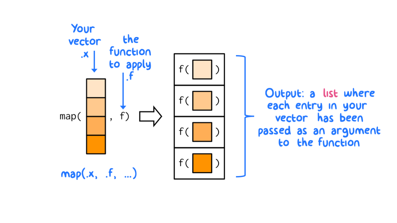
Figure 8.1: The map functions transform their input by applying a function to each element of a list or atomic vector and returning an object of the same length as the input.
As shown above in Figure 8.1, the generic form of map() always returns a list object as the output (thanks to Hadley Wickham for the graphic). A list is a generic vector that can contain multiple objects (other vectors, data frames, etc.). Indeed, a data frame (and a tibble) is a special kind of list: a data frame is a list of vectors (columns) of equal length. A data frame can contain different vector objects but those objects must be placed in separate columns and each column vector must be the same length (when all the columns are equal length that means that data frames are rectangular lists). A generic list does not need to be rectangular because generic list entries are more distinct. Further, a list can contain another list (like a set of small boxes that are nested within a larger box). Think of a list like a drawer organizer - it can contain lots of different objects, all of which might be related to another in some way or, at least, might be used together for some common purpose. To review:
- A vector is a one-dimensional object where all the entries are the same type.
- A matrix is a two-dimensional (rectangular) object where all entries are the same type, but ordered into rows and column indices.
- A data frame is a two dimensional (rectangular) object that contains columns of different vectors. The type of vector (e.g.,
character,numeric,logical, etc.) can differ from one column to the next but all entries within each vector column must be the same. - A list can contain different vector objects of different types and different lengths. A list can also contain other lists. A list does not need to be rectangular.
To illustrate the versatility of lists, let’s create one that contains a numeric vector, a matrix, and a data frame.
my.chr.vector <- c("Harry", "Ron", "Hermione", "Draco")

my.num.matrix <- matrix(data = 1:20, nrow=5)

my.df <- slice_sample(.data = mpg, n=7)

my.list <- list("entry_1" = my.chr.vector,
                "entry_2" = my.num.matrix,
                "entry_3" = my.df)

glimpse(my.list)
## List of 3
## $ entry_1: chr [1:4] "Harry" "Ron" "Hermione" "Draco"
## $ entry_2: int [1:5, 1:4] 1 2 3 4 5 6 7 8 9 10 ...
## $ entry_3: tibble [7 × 11] (S3: tbl_df/tbl/data.frame)
## ..$ manufacturer: chr [1:7] "ford" "honda" "dodge" "honda" ...
## ..$ model : chr [1:7] "explorer 4wd" "civic" "dakota pickup 4wd" "civic" ...
## ..$ displ : num [1:7] 4.6 1.6 4.7 1.6 3.7 3.8 5.3
## ..$ year : int [1:7] 2008 1999 2008 1999 2008 1999 2008
## ..$ cyl : int [1:7] 8 4 8 4 6 6 8
## ..$ trans : chr [1:7] "auto(l6)" "manual(m5)" "auto(l5)" "manual(m5)" ...
## ..$ drv : chr [1:7] "4" "f" "4" "f" ...
## ..$ cty : int [1:7] 13 28 14 25 15 16 16
## ..$ hwy : int [1:7] 19 33 19 32 19 26 25
## ..$ fl : chr [1:7] "r" "r" "r" "r" ...
## ..$ class : chr [1:7] "suv" "subcompact" "pickup" "subcompact" ...Lists can be accessed in similar ways to vectors. For example, by using single-bracket indexing, [ ], a list element is returned.
## $entry_1
## [1] "Harry"    "Ron"      "Hermione" "Draco"
Note that “single bracket” indexing returns a “list element” of class: list.
## [1] "list"If you want access to the vector contents of the list element, you can use the $ symbol to access the contents of each list entry, or, you can use “double bracket” indexing, [[ ]]:
## [1] "Harry" "Ron" "Hermione" "Draco"## [1] "character"## [,1] [,2] [,3] [,4]
## [1,] 1 6 11 16
## [2,] 2 7 12 17
## [3,] 3 8 13 18
## [4,] 4 9 14 19
## [5,] 5 10 15 20## [1] "matrix" "array"Working with lists is one of the mental hurdles to overcome when learning map(). However, there are variants in the map_ family of functions that return simpler object types; we will work with these simplified functions to begin.
Purrr:: Function |
Object Type Returned |
|---|---|
| map() | list |
| map_lgl() | logical |
| map_int() | integer |
| map_dbl() | numeric |
| map_chr() | character |
| map_dfr() | data frame (output by row-binding) |
| map_dfc() | data frame (output by column-binding) |
Let’s use map_dfr() to apply our function, import.w.name(), onto the vector of file names and paths (file_list). The “r” in map_dfr() means that the resultant data frame output by map_ will be created by binding rows together as the function moves down each index in the file list. This is shown schematically in Figure 8.2 below.
file_list <- list.files('./data/purpleair/', full.names=TRUE)

# map the import.w.name() function to all objects within `file_list` sequentially
# and combining the result into a single data frame with row binding
PA_data_merged <- map_dfr(file_list, import.w.name)

glimpse(PA_data_merged)
## Rows: 6,371
## Columns: 6
## $ datetime <dttm> 2018-10-22 17:52:21, 2018-10-22 17:53:41, 2018-10-22…
## $ current_temp_f <dbl> 90, 86, 87, 87, 87, 87, 86, 86, 86, 86, 86, 86, 86, 8…
## $ current_humidity <dbl> 12, 13, 13, 13, 13, 13, 12, 13, 13, 13, 13, 13, 13, 1…
## $ pressure <dbl> 851.66, 851.68, 851.56, 851.59, 851.54, 851.57, 851.5…
## $ pm2_5_atm <dbl> 2.45, 3.43, 2.76, 2.00, 1.82, 1.98, 1.95, 2.48, 2.27,…
## $ sensor_ID <chr> "PA019", "PA019", "PA019", "PA019", "PA019", "PA019",…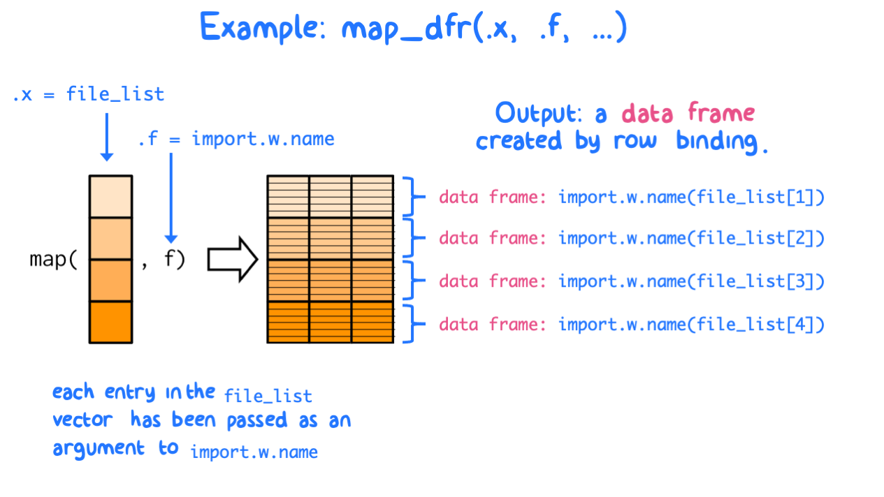
Figure 8.2: Example: using map_dfr() to import a file list using a custom function
8.5 Applying functions to multiple columns: dplyr::across()
There are many instances where you will want to apply a function to several columns in a data frame, often in conjunction with mutate() or summarise(). The across() function helps you do this efficiently, by applying a function across various column variables in a data frame.
The across() function has two required arguments: the column variables being treated (.cols =) and the function(s) being applied to those columns (.fns =). For example, if you wanted to change the cyl, drv, and class variables in the mpg data frame to factors, you could use:
Before providing more examples of across(), it’s worth taking a tangent to discuss more efficient ways to select multiple columns beyong using c().
8.5.1 Using <tidy-select> syntax to select columns
Many of the dplyr:: functions support Tidy Selection as a means to choose certain column variables when operating on a data frame. For example, maybe you want to choose only columns whose names start with a common prefix (starts_with()) or whose names contain a common string (contains()). The <tidy-select> helpers provide syntax for efficiently specifying your .cols = argument in R. These helpers, shown below, can be used as column/variable selection arguments whenever you see the text <tidy-select> in the function’s help file.
| Helper | Explanation | Example |
|---|---|---|
| everything() | Matches all variables | rename_with(mpg, .cols = everything(), .fn = toupper)) |
| starts_with() | Starts with a prefix | select(mpg, starts_with(‘c’)) |
| ends_with() | Ends with a suffix | mutate(mpg, across(ends_with(‘y’), .fns = ~0.425*.x, .names = ‘km_per_liter_{.col}’)) |
| contains() | Contains a literal string | summarise(mpg, across(contains(‘y’), .fns = mean, .names = ‘mean_{.col}’)) |
| matches() | Matches a regular expression | rename_with(mpg, .cols = matches(‘y$’), .fn = toupper) |
| where() | Selects variables if function returns TRUE | select(mpg, where(is.numeric)) |
| if_any() | Filters rows if function returns TRUE | filter(if_any(everything(), is.character)) |
There are also helper symbols that can be used (an in conjunction with the helper verbs above) to make selections. For example, if you wanted to keep all columns except for those containing logical vectors, you could use select(data = .x, !where(is.logical)). These symbols are outlined in the table below. For further reference, see this help page.
| Symbol | Explanation | Example (mpg dataframe) |
|---|---|---|
| : | for selecting a range of consecutive columns | model:year |
| ! | for taking the complement of a set of variables | !where(is.numeric) |
| & | for selecting the intersection of two sets of variables | where(is.numeric) & contains(“y”) |
| | | for selecting the union of two sets of variables | where(is.numeric) | starts_with(“m”) |
| c() | for combining selections | !c(Make, hwy) |
8.5.2 Examples dplyr::across()
Perform unit conversions:
# convert the cty and hwy variables in the mpg data frame to km/l
mutate(mpg, across(ends_with("y"), # select cty and hwy
                   .fns = ~0.425*.x, # unit conversion m/gal to km/l
                   .names = "km_per_liter_{.col}")) %>% # how to name new columns
  # select first 2 cols and those containing strings indicated
  select(1:2 | contains("year") | contains("km")) %>%
  slice_sample(n=5)
## # A tibble: 5 × 5
## manufacturer model year km_per_liter_cty km_per_liter_hwy
## <chr> <chr> <int> <dbl> <dbl>
## 1 honda civic 1999 11.9 14.0
## 2 volkswagen jetta 1999 8.07 11.0
## 3 ford explorer 4wd 2008 5.52 8.07
## 4 toyota toyota tacoma 4wd 1999 6.38 8.07
## 5 toyota camry solara 1999 8.92 11.5Summarizing the data range for only the numeric vectors:
# show the ranges of all numeric vectors in the mpg data frame
mpg %>%
  summarise(across(where(is.numeric), .fns = range))
## # A tibble: 2 × 5
## displ year cyl cty hwy
## <dbl> <int> <int> <int> <int>
## 1 1.6 1999 4 9 12
## 2 7 2008 8 35 448.5.3 Anonymous Functions
Sometimes, we want to do some pre-processing of our data before a summary call. In the case below, we summarize (by count) the number of NA values in a data frame for each column of the data frame (this is a great quality control check for new data). To do this, we apply the is.na() function to each entry, then sum them up by row (because is.na returns logical TRUE/FALSE objects that equate to 1 or 0, respectively).
We can get across() to achieve this by creating a custom one-time function as shown in the code below. Such custom functions are known as anonymous functions because they doesn’t have an assigned function name. See example below, where we define a quick, one-time function as the .fns = argument in across():
# sum up the number of NAs by column in a data frame
# create a custom function within the across() function
# note that everything() is a tidyselect verb from above
mpg %>%
  summarise(across(everything(),
                   .fns = function(x) sum(is.na(x))))
## # A tibble: 1 × 11
## manufacturer model displ year cyl trans drv cty hwy fl class
## <int> <int> <int> <int> <int> <int> <int> <int> <int> <int> <int>
## 1 0 0 0 0 0 0 0 0 0 0 0Anonymous functions are useful once you get used to the idea of “creating a function within a function”. They are common when you only need to use a function once. You will often see them written in their shorthand form (using the ~ symbol and .x) as shown below. Essentially, the ~ symbol tells R to expect either a function with multiple arguments or a chain of functions (i.e., some pre-processing of the data). The .x is a placeholder for the argument of your function.