Chapter 6 Strings, Dates, and Tidying
6.1 Chapter 6 Objectives
This Chapter is designed around the following learning objectives. Upon completing this Chapter, you should be able to:
- Define the meaning of “strings” and “date time” objects in R
- Manipulate character strings using the
stringrandtidyrpackages of functions - Parse strings using regular expressions (“regex”)
- Describe how R stores a POSIXct date and time object internally
- Convert a character vector to a date format using functions from the
lubridateR package - Extract information from a date object (e.g., month, year, day of week) using
lubridatefunctions - Search, organize, and visualize data that are linked to date objects
- Apply functions from the
dplyrandtidyrpackages to make dataframes “tidy”
6.2 Strings
Strings are a form of character data like “John”, or “blue”, or “John’s sample 8021A turned blue”.
Strings are defined in R using quotes " " and stored as character
vectors; they often show up in data analysis in one of two ways:
As metadata. Metadata means: “data that describe other data”.
A readme.txt file is metadata; notes and code comments are metadata. All of these types of data usually come in the form of strings and are included with the data your are analyzing but not in the dataset itself.As vectorized data. In R programming, “vectorized” means: stored as a column of data. Examples of vectorized strings that you might find include things like: “participant names”, or “survey responses to question 1”, or “mode of failure”. The example below creates three different string vectors in R. Note: You can check the type of object you’ve created using the
class()ortypeof()functions.
# examples of vectorized string data
names_respond <- c("Ahmed",
                   "Josh",
                   "Mateo",
                   "William",
                   "Ali",
                   "Wei",
                   "Steve-O",
                   "John")
q1_responses <- c("Because you told me to do it.",
                  "It seemed like the right thing to do at the time.",
                  "Because I had been over-served.",
                  "I don't know. I just did it.",
                  "I got caught up in the heat of the moment.",
                  "I was given an opportunity. I took my shot.",
                  "I plead the 5th.",
                  "I could ask you the same question.")
failure_mode <- c("fracture",
                  "yielding",
                  "deflection",
                  "fatigue",
                  "creep")

# proof of vector type
class(names_respond)
## [1] "character"The first step in analyzing a string is to parse it. To parse means to examine the individual components. For example, when you read this sentence you parse the words and then assign meaning to those words based on your memory, your understanding of grammar, and the context in which those words occur. Context is often critical to understanding because the meaning of words can change from one context to the next (i.e., whether you are reading an instruction manual, a text message, a novel, or a warrant for your arrest). Strings can be challenging to analyze because computers are built on logical operations and mathematics; strings are neither of those. Computers have fantastic memory, are OK at grammar, and are comically poor at contextualization. Taken together, this means that strings can be challenging (but not impossible) to analyze using computers.
Are you active on social media platforms like Instagram or Twitter? You can bet that a computer program has downloaded and parsed all of your posts, each one as a string. You can learn a lot about a person (and their buying habits) from what they post online!
In this chapter, we will introduce a few simple string functions from base R
and the stringr package. We will also introduce the concept of
regular expressions as a means to perform more advanced string
manipulation.
6.2.1 String detect, match, subset
One of the simplest string operations is to search whether a string contains a
pattern of interest. The stringr package (part of the
Tidyverse) was developed
to simplify the
analysis of strings. Most of the functions in stringr begin with str_ and
end with a specific function name. A full list of functions is provided
here. Some examples:
str_detect()returns a vector of logical values (TRUE/FALSE) indicating whether the pattern was detected within each string searched. The function takes two arguments, thestringto be searched and thepatternfor which to search. Let’s search for the pattern"Josh"in the character vector of strings,names_respond, that we created above:
## [1] FALSE TRUE FALSE FALSE FALSE FALSE FALSE FALSEAs expected, only one string in the vector produced a match.
An added benefit of logical functions like str_detect() is that return values
of TRUE are coded as 1 and FALSE as 0. Thus, if we sum() the result of
the str_detect() search, we will get the cumulative number of matches to
"Josh" from within our data.
## [1] 1In other words, logical functions like str_detect() allow us to do math on
string data! For example, we can now calculate the proportion of "Josh"
entries within our sample:
## [1] 0.125str_extract()takes the same arguments asstr_detect()but returns a vector of the matched values (by string index). By “matched values”, I mean only the portion of the string for which the search created a match.
## [1] NA "Jo" NA NA NA NA NA "Jo"str_subset()returns only the entries that were matched (i.e., if a match was detected, then the entire string that was matched is returned). If we subset our short list of names to the pattern of letters"li", we get:
## [1] "William" "Ali"To note, there are base R versions of all these stringr functions. Most are
performed with the grep family of functions. The term “grep” is an acronym
for Global Regular Expression Pattern (more on
regular expressions below). Many “old-school” coders use this family of
functions, therefore, you will encounter them in the wild, so it’s worth
knowing about them.
| stringr_funcs | base_funcs |
|---|---|
| str_detect(x, pattern) | grepl(pattern, x) |
| str_match(x, pattern) | regexec(pattern, x) + regmatches() |
| str_subset(x, pattern) | grep(pattern, x, value = TRUE) |
6.2.2 Regular Expressions
Before going much farther, we should spend some time discussing
regular expressions or regex for short. When we pass a pattern
argument to a function like str_detect(), the function treats that argument
like a “regex”. Up until this point, I have only passed simple character
strings as pattern arguments (i.e., pattern = "Josh"). In reality, we can
create much more advanced search criteria using regex syntax within our
search patterns.
A regular expression is a sequence of characters that define a search pattern to be implemented on a string.
In the R programming language, regular expressions follow the POSIX 1003.2
standard; regex can have different syntax based on the underlying standard.
Regex are created by including search syntax (i.e., symbols that communicate
search parameters) within your quoted string. For example, square brackets []
in a search pattern indicate a search for any of the characters within the
brackets; conversely, to match all the characters you simply include them in
quotes. A key strength of regex patterns is that they allow you to use logical
and conditional relations. For example, the following text search patterns can
be coded as regex:
| Desired Search Pattern | Regex in R |
|---|---|
| any letter followed by the numbers 3, 4, or 5 | “[:alpha:][345]” |
| strings that start with ‘ID’ and are followed by 4 numbers | “^ID[:digit:]{4}” |
One challenging aspect of string searching in R, however, is that certain
“special characters” like the quote " and the backslash \ symbol must be
explicitly identified within the string in order to be interpreted by R
correctly. To identify these special characters in a string, you need to
“escape” that character using a backslash \. Thus, if you want to
search for a quote symbol, you would type in \". Whenever a regex requires
the use of a \, you have to identify it within a string as \\. The table
below shows some basic regex syntax and how they would be implemented as a
search pattern in R.
| Regex syntax | String to be matched | Example in R |
|---|---|---|
| \d | Any numeric digit | “\\d” or “[:digit:]” |
| [abc] | matches a, b, or c | “[abc]” |
| [a-z] | matches every character between a and z | “[a-z]” |
| [^abc] | matches anything except a, b, or c | “[^abc]” |
| (abc) | creates a “capture group” whereby abc must occur together | “(abc)” |
| ^b | starts with: look for “b” at the start of a string | “^b” |
| b$ | ends with: look for “b” at the end of a string | “b$” |
| a|b | match a or b | “a|b” |
Regex sequences have seemingly no end of sophistication and nuance; you
could spend dozens of hours learning to use them and hundreds more learning to
master them. We will only introduce basic concepts here. More in-depth
introductions to regex syntax and usage can be found on Hadley Wickham’s R course,
on the stringr
cheatsheet
developed by RStudio, and through practice with, my personal favorite, a game
of Regex Golf.
6.2.3 String split, replace
str_split() will split a string into two (or more) pieces when a match is
detected. The string will always be split at the first match and again at each
additional match location, unless you specify that only a finite number of n
matches should occur. A couple points to note:
str_split()splits on each side of the match; the matched part of the string is not included in the output.because both sides of the split string are returned, your output will take the form of a
list.
## [[1]]
## [1] "Ahmed"
##
## [[2]]
## [1] "Josh"
##
## [[3]]
## [1] "Ma" "eo"
##
## [[4]]
## [1] "William"
##
## [[5]]
## [1] "Ali"
##
## [[6]]
## [1] "Wei"
##
## [[7]]
## [1] "S"     "eve-O"
##
## [[8]]
## [1] "John"
str_replace() searches for a match and then replaces the matched value
with a new string of your choosing. The function takes three arguments: the
string to be searched, the pattern to match, and the replacement
string to be inserted. Let’s replace the first period detected in each of
the q1_responses strings with a question mark. Both . and ? are
special characters so we need to “escape” each of these symbols with two
back-slashes \\.
## [1] "Because you told me to do it?"
## [2] "It seemed like the right thing to do at the time?"
## [3] "Because I had been over-served?"
## [4] "I don't know? I just did it."
## [5] "I got caught up in the heat of the moment?"
## [6] "I was given an opportunity? I took my shot."
## [7] "I plead the 5th?"
## [8] "I could ask you the same question?"
The str_replace() family of functions is useful for cleaning up misspellings
(or other unwanted language) in strings. Note, however, that str_replace()
will normally replace only one instance of a match; use str_replace_all() if
you plan to encounter multiple matches that need replacing.
The pattern = argument for matching can be a single
string or a vector of strings. In the latter case, you can define a
vector of keywords that you might be searching for across
sentences. In that case, use
pattern = c(“pattern_1”, “pattern_2”, “pattern_3”, …etc).
6.3 Dates and Date-times
Working with dates and times can be challenging. This section begins with a
discussion of how base R handles dates and times, since there is a ton of code
out there that utilizes these older functions. We will then quickly transition
to the lubridate family of functions (part of the Tidyverse) because of their
versatility and ease-of-use.
6.3.1 Dates and Times in base R
Dates and times in base R all proceed from an “epoch” or time origin. In R, the epoch or “dawn of time” occurred at midnight on January 1st, 1970. For the sake of the R programming world, the concept of time started at that precise moment and has moved forward ever since. To note: R can handle date-times before 1/1/1970; it just treats them as negative values!
To see a date-time object, you can tell R to give you the current “System Time”
by calling the Sys.time() function.
## [1] "2025-11-17 11:10:31 MST"As you can see, we got back the date, time, and timezone used by my computer
(whenever I last ran this code in bookdown). If you want to see how this
time is stored in R internally, you can use unclass(), which returns an
object value with its class attributes removed. When we wrap unclass()
around Sys.time(), we will see the number of seconds that have occurred
between the epoch of 1/1/1970 and right now:
## [1] 1763403032That’s a lot of seconds. How many years is that?
Just divide that number by [60s/min \(\cdot\) 60min/hr \(\cdot\) 24hr/d \(\cdot\)
365d/yr] => 55.9171433 years.
This calculation ignores leap years, but you get the point…
6.3.2 Date-time formats
Note that the Sys.time() function provided the date in a
“year-month-day” format and the time in an “hour-minute-second”
format: 2025-11-17 11:10:31.950992.
Not everyone uses this exact ordering when they record dates and times, which is one of the reasons working with dates and times can be tricky. You probably have little difficulty recognizing the following date-time objects as equivalent but, for some computer programs, not so much:
| 12/1/99 8:46 PM |
| 1-Dec-1999 20:46 UTC |
| December 1st, 1999, 20:46:00 |
You will often see time followed by “UTC”, which stands for “Universal Time, Coordinated”. UTC is preferred by programmers because it doesn’t have a timezone and it doesn’t follow Daylight Savings Time conventions. Daylight savings is the bane of many coders.
In practice, UTC is the same time as GMT (Greenwich Mean Time, pronounced “gren-itch”) but with an important distinction. GMT is one of the many time-zones laid out across Earth’s longitude, whereas, UTC has no timezone; UTC is the same time for everyone, everywhere.
In Colorado, we are UTC-6 hours during daylight savings (March-Nov) and UTC-7 during standard time (Nov-March). This means that most Coloradoans eat dinner at 12am UTC (6pm MST).
6.3.3 Date-time classes in R
R has several classes of date-time objects, none of which are easy to remember:
POSIXct- stored as the time, in seconds, between theepochof 1970-01-01 00:00:00 UTC and the date-time object in question.- the ‘ct’ stands for “continuous time” to represent “continuous seconds from origin”;
- A
POSIXctobject is a single numeric vector, thus useful for efficient computing.
POSIXlt- stored as a list of date-time objects.- the ‘lt’ stands for “list time”.
- A
POSIXltlist contains the following elements:- sec as 0–61 seconds
- min as 0–59 minutes
- hour as 0–23 hours
- mday as 1–31 day of the month
- mon as 0–11 months after the first of the year
- year as Years since 1900
- wday as 0–6 day of the week, starting on Sunday
- yday as 0–365 days of the year.
- isdst as a flag for Daylight savings time. Positive if in force, zero if not, negative if unknown.
POSIXt- this is a virtual class.POSIXt(without the “l”) is an internal way for R to convert betweenPOSIXctandPOSIXltdate-time objects.- Think of the
POSIXtas a way for R to perform operations/conversions between aPOSIXctandPOSIXltobject without throwing an error your way.
- Think of the
As a reminder, here are some common object classes in R:
| Class | Example |
|---|---|
character
|
“Chemistry”, “Physics”, “Mathematics” |
numeric
|
10, 20, 30, 40 |
factor
|
Male [underlying number: 1], Female [2] |
Date
|
“2010-01-01” [underlying number: 14,610] |
logical
|
TRUE, FALSE |
date-time
|
“2020-06-23 11:05:20 MDT” |
To discover the class of a vector (including a column in a dataframe—remember
each column can be thought of as a vector), you can use class():
## [1] "POSIXct" "POSIXt"Both the POSIXct and POSIXlt class of objects return the same value to the
user; the difference is really in how these classes store date-time objects
internally. To examine them, you can coerce Sys.time() into each of the two
classes using as.POSIXct and as.POSIXlt functions and then examine their
attributes.
## [1] 1763403032time_now_lt <- as.POSIXlt(Sys.time())
str(unclass(time_now_lt)) # the `str()` function makes the output more compact## List of 11
## $ sec : num 32
## $ min : int 10
## $ hour : int 11
## $ mday : int 17
## $ mon : int 10
## $ year : int 125
## $ wday : int 1
## $ yday : int 320
## $ isdst : int 0
## $ zone : chr "MST"
## $ gmtoff: int -25200
## - attr(*, "tzone")= chr [1:3] "" "MST" "MDT"
## - attr(*, "balanced")= logi TRUEIt’s easy to see why the POSIXct object class is more computationally
efficient, but it’s also nice to see all the date-time information packed into
the POSIXlt. This is why R keeps a key to unlock both using POSIXt.
As my father used to say: clear as mud?
6.3.4 Reading and classifying date-times
Oftentimes, when data is read into R, there are column elements that contain
date and time information. These dates and times are often interpreted by R
as character vectors, which means they have lost their relational attributes.
For example, you cannot subtract “Monday 08:00” from “Wednesday 12:00” and get
“2 days 4 hours”. If we want to analyze dates and times in a relational way,
we need to instruct R to recognize these as date-time objects (i.e., as either
the POSIXct or POSIXlt class). Thus, to convert a character vector into
date or date-time object requires a change of that vector’s class.
Date-time elements can be tricky to work with for a few reasons:
- Different programs store and handle dates and times in different ways
- The existence of time zones means that date-time values can change with location
- Date-time strings can be separated with spaces, colons, commas, slashes, dashes, or a mix of all those together (see Table 6.2)
The base R function to convert between character classes and date-time
classes is the function strptime(), which is short for
“string parse into date-time”. I mention this function not because
I encourage you to use it but because I want you to be able to recognize it. The
function has over 39 conversion specifications that it can take as arguments.
That is to say, this function not simple to master. If you are a glutton for
punishment, I invite you to read the R Documentation with ?strptime.
Here are a few base R functions for working with date-time objects that are worth knowing:
| {base} R Function | Value Returned | Example |
|---|---|---|
| Sys.Date() | Current system date | “2020-06-23” |
| Sys.time() | Current system date-Time | “2020-06-23 11:05:20 MDT” |
| Sys.timezone() | Current system timezone | “America/Denver” |
| as.POSIXct() | date-time object of class POSIXct | “2020-06-23 11:05:20 MDT” |
| as.POSIXlt() | date-time object of class POSIXlt | “2020-06-23 11:05:20 MDT” |
| strptime() | date-time object of class POSIXlt | “2020-06-23 11:05:20 MDT” |
6.4 lubridate
The lubridate package was developed specifically to make it easier to work
with date-time objects. You can find out more information on lubridate
here.
6.4.1 Parsing functions in lubridate
One of best aspects of lubridate is its ability to parse date-time objects
with simplicity and ease; the lubridate parsing functions are designed as
“named-to-order”. Let me explain:
Parse: to break apart and analyze the individual components of something, like a character string.
If a character vector is written in “year-month-day” format (e.g.,
"2020-Dec-18"), then thelubridatefunction to convert that vector isymd().If a character vector is written in “day-month-year” format (e.g.,
"18-Dec-2020"), then thelubridatefunction to convert that vector isdmy(). Try it out:
# create a character vector
date_old <- "2020-Dec-18"

# prove it's a character class
class(date_old)
## [1] "character"# convert it to a `Date` class with `ymd()`
date_new <- lubridate::ymd(date_old)
# prove it worked
class(date_new)## [1] "Date"That little conversion exercise may not have blown you away, but watch what
happens when I feed the following set of wacky character vectors into that
same lubridate parsing function, ymd():
messy_dates <- c("2020------Dec the 12",
                 "20.-.12.-.12",
                 "2020aaa12aaa12",
                 "20,12,12",
                 "2020x12-12",
                 "2020   ....    12        ......     12",
                 "'20.December-12")
ymd(messy_dates)
## [1] "2020-12-12" "2020-12-12" "2020-12-12" "2020-12-12" "2020-12-12"
## [6] "2020-12-12" "2020-12-12"Boom. That’s right, the ymd() parsing function figured them all out correctly
with almost no effort on your part. But wait, there’s more!
The lubridate package contains parsing functions for almost any order you can
imagine.
| Parsing Function | Format to Convert |
|---|---|
ymd()
|
year-month-day |
mdy()
|
month-day-year |
dmy()
|
day-month-year |
And if you need to parse a time component, simply add a combination of _hms to
the function call to parse time in “hours-minutes-seconds” format. Some
additional examples of how you would parse time that followed from a ymd
format:
| Parsing Function | Format to Convert |
|---|---|
ymd_h()
|
year-month-day_hours |
mdy_hm()
|
year-month-day_hours-minutes |
dmy_hms()
|
year-month-day_hours-minutes-seconds |
The beauty of the lubridate parsers is that they do the hard work of cleaning
up the character vector, regardless of separators or delimiters within each
string, and return either a Date or Date-time object class.
6.4.2 Date-time manipulation with lubridate
To convert the date column in the daily_show data into a Date class, you can
run:
library(package = "lubridate")

# check the class of the 'date' column before mutating it
class(x = daily_show$date)
## [1] "character"## # A tibble: 3 × 5
## year job date category guest_name
## <dbl> <chr> <date> <chr> <chr>
## 1 1999 actor 1999-01-11 Acting Michael J. Fox
## 2 1999 Comedian 1999-01-12 Comedy Sandra Bernhard
## 3 1999 television actress 1999-01-13 Acting Tracey Ullman## [1] "Date"Once you have an object in the Date class, you can do things like plot by
date, calculate the range of dates, and calculate the total number of days the
dataset covers:
# report the min and max dates
range(daily_show$date)

# calculate the duration from first to last date using base
max(daily_show$date) - min(daily_show$date)
We could have used these to transform the date in daily_show, using the
following pipe chain:
daily_show <- readr::read_csv(file = "data/daily_show_guests.csv",
                              skip = 4) %>%
  dplyr::rename(job = GoogleKnowlege_Occupation,
                date = Show,
                category = Group,
                guest_name = Raw_Guest_List) %>%
  dplyr::select(-YEAR) %>%
  dplyr::mutate(date = lubridate::mdy(date)) %>%
  dplyr::filter(category == "Science")

# show first two rows of dataframe
head(x = daily_show, n = 2)
## # A tibble: 2 × 4
## job date category guest_name
## <chr> <date> <chr> <chr>
## 1 neurosurgeon 2003-04-28 Science Dr Sanjay Gupta
## 2 scientist 2004-01-13 Science Catherine WeitzThe lubridate package also includes functions to pull out certain elements of
a date, including:
wday()return the day of the week pertaining to a Date objectmday()return the day of the month pertaining to a Date objectyday()return the day of the year pertaining to a Date objectmonth()return the month pertaining to a Date objectquarter()return the quarter of hte year pertaining to a Date objectyear()return the year pertaining to a date object
For example, we could use wday() to create a new column with the weekday of
each show:
daily_show %>%
  dplyr::mutate(show_day = lubridate::wday(x = date,
                                           label = TRUE)) %>%
  dplyr::select(date, show_day, guest_name) %>%
  dplyr::slice(1:5)
## # A tibble: 5 × 3
## date show_day guest_name
## <date> <ord> <chr>
## 1 2003-04-28 Mon Dr Sanjay Gupta
## 2 2004-01-13 Tue Catherine Weitz
## 3 2004-06-15 Tue Hassan Ibrahim
## 4 2005-09-06 Tue Dr. Marc Siegel
## 5 2006-02-13 Mon Astronaut Mike Mullane
R functions tend to use the timezone of YOUR
computer’s operating system by default—or UTC, or GMT. You need to be
careful when working with dates and times to either specify the time
zone or convince yourself the default behavior works for your
application. To see or set your computer’s time zone, use the
Sys.timezone() function from {base}.
6.5 Tidy Data
“Tidy Data” is a philosophy for how to arrange your data in a intuitive,
rectangular fashion, commonly in a dataframe. In his
2014 paper,
Hadley Wickham states,
“tidy datasets provide a standardized way to link the structure of a dataset (its physical layout) with its semantics (its meaning).”
The definition of a tidy dataset is straightforward:
- Each variable forms a column.
- Each observation forms a row.
- Each type of observational unit forms a table.
The first two rules, each variable forms a column and each observation forms a row, are relatively easy to implement. In fact, most of the dataframes that we have used so far follow this convention. The trick is to note that some column variables might look independent from one another, when, in fact, the columns represent a single variable broken out by some hierarchical, or nesting, structure.
For example, the (untidy) table below (6.6) shows exam
grades for three students. Table 6.6 is untidy because
the variable depicting the exam score shows up in three different columns.
Another way to characterize the untidiness of this table is that we have three
different exams (Exam1, Exam2, Exam3) that represent a variable (Exam_# or
Exam_type), that is not represented with a column.
| Name | Exam1_Score | Exam2_Score | Exam3_Score |
|---|---|---|---|
| Harry | 85 | 79 | 88 |
| Ron | 81 | 75 | 89 |
| Hermione | 95 | 97 | 99 |
Thus, to tidy table 6.6, we need to create a variable
called Exam and move all the scores into a new column vector named Scores.
This effectively makes the data “long” rather than “wide”.
| Name | Exam | Scores |
|---|---|---|
| Harry | 1 | 85 |
| Harry | 2 | 81 |
| Harry | 3 | 95 |
| Ron | 1 | 79 |
| Ron | 2 | 75 |
| Ron | 3 | 97 |
| Hermione | 1 | 88 |
| Hermione | 2 | 89 |
| Hermione | 3 | 99 |
For our work, one of the goals of data cleaning is to create datasets that
follow this tidy convention. Fortunately, the tidyr package contains a
useful function called pivot_longer() for re-arranging dataframes from
untidy (typically “wide) to tidy (”long”).
pivot_longer() is designed to “lengthen” a data frame by
“increasing the number of rows and decreasing the number of columns”.
This function creates two new columns as output and requires four arguments:
data =the dataframe to be lengthenedcols =a list of the columns that should be combined together (forming a single variable to be represented in a new, single column)names_to= this is an output column that contains the names of the old columns that are being combined.values_to= this is the other output column that contains the values from within the old columns that are being combined.
The pivot_longer() function always creates two new
columns:
-
one column contains
names_to =information. -
the other column contains the
values_to =data.
In the case of Table 6.6, we are using cols = to combine
Exam1_Score, Exam2_Score and Exam3_Score into a a column of
names_to = "Exam" and the data represented in those three columns gets moved
into a column of values_to = "Scores". We also add a call to dplyr::mutate()
and dplyr::case_when() to convert strings to numbers.
The case_when() function allows you introduce multiple “if/else” statements into
a vectorized operation, such as within this call to dplyr:mutate(). This function
takes a series of logical arguments as cases, with each case seeking to find a “match”. Once a “match” occurs, an outcome instruction is followed. In the code
chunk below, the left-hand-side of each “case” evaluates whether each entry in
the Exam column equates to a particular string (like "Exam_1_Score"). On the
right-hand-side of each case, separated by a tilde ~, contains the mutate()
instruction. In plain speak, the function reads:
If the vector contains a string that matches “Exam_1_Score”, then replace that entry with a 1; else, if the vector contains a string that matches “Exam_2_Score”, then replace that entry with a 2; else, if the vector contains a string that matches “Exam_3_Score”, then replace that entry with a 3.
grades_untidy <- tibble::tibble(
  Name = c("Harry", "Ron", "Hermione"),
  Exam1_Score = c(85, 81, 95),
  Exam2_Score = c(79, 75, 97),
  Exam3_Score = c(88, 89, 99)
  )

tidygrades <- tidyr::pivot_longer(data = grades_untidy,
                                  cols = Exam1_Score:Exam3_Score,
                                  names_to = "Exam",
                                  values_to = "Scores") %>%
  dplyr::mutate(Exam = dplyr::case_when(
    Exam == "Exam1_Score" ~ 1,
    Exam == "Exam2_Score" ~ 2,
    Exam == "Exam3_Score" ~ 3
))| Name | Exam | Scores |
|---|---|---|
| Harry | 1 | 85 |
| Harry | 2 | 79 |
| Harry | 3 | 88 |
| Ron | 1 | 81 |
| Ron | 2 | 75 |
| Ron | 3 | 89 |
| Hermione | 1 | 95 |
| Hermione | 2 | 97 |
| Hermione | 3 | 99 |
Now these data are tidy, wherein each variable forms a column, each row forms an observation, and the table is specific to one observational unit. This may seem obvious, but most data analysis problems occur because of poor data management techniques. Remember: What might seem useful at the time—like a color-coded Excel spreadsheet—is a pain for computers and not reproducible. Do yourself a favor and begin with the end in mind: tidy data.
6.6 Chapter 6 Exercises
The following exercises use data on tweets from United Senators, processed by FiveThirtyEight.
6.6.1 Set 1: Data import and manipulation
Create a pipeline that
- imports the raw data (.csv) containing tweets from all US senators,
- filters the raw data to only Colorado (“CO”) senators,
- creates 4 new variables within a call to the appropriate
dplyrfunction and four distinctlubridatefunctions based on the format of the date or date-time variable:datefromcreated_athour_cofromdate, also setting “America/Denver” timezone withlubridate::with_tzone()monthfromdateweekfromdate, and
- retains all variables except
url,created_at, andbioguide_id
# pipeline to import, filter, manipulate datetime vars, select vars
tweets_co <- readr::read_csv("data/senators.csv") %>%
  dplyr::filter(state == "CO") %>% # filter to Colorado senators
  dplyr::mutate(date = lubridate::mdy_hm(created_at), # convert timestamp to datetime object
         hour_co = lubridate::hour(lubridate::with_tz(date, # convert timestamp to datetime object
                                                      tzone = "America/Denver")), # and add timezone label
         month = lubridate::month(date), # create var of month from timestamp
         week = lubridate::week(date)) %>% # create var of week from timestamp
  dplyr::select(-(c(url, created_at, bioguide_id))) # retain all vars except 3
6.6.2 Set 2: Counting
- Which Colorado senators are included in the data?
# find unique strings within user variable
# if you convert to factor, you can also find `levels()`
unique(tweets_co$user)
## [1] "SenBennetCO" "SenCoryGardner"- Which Colorado Senator tweets the most?
# compare number of tweets by senator; remember to always ungroup grouped data!
tweets_co %>%
  dplyr::group_by(user) %>%
  dplyr::tally() %>%
  dplyr::ungroup()
## # A tibble: 2 × 2
## user n
## <chr> <int>
## 1 SenBennetCO 2211
## 2 SenCoryGardner 32256.6.3 Set 3: Weekly tweets
Create a time series plot that indicates tweet activity on a weekly basis since 2011 for the Colorado senators. You will need to first create a new data frame that contains new time-date variables based on the (a) total time and (b) weeks since data collection started.
# create new time-based variables
tweets_co_wk <- tweets_co %>%
  dplyr::mutate(time_since = as.duration(date - min(date)), # create duration variable, time since first datum
         week = round(as.numeric(time_since, "weeks"), 0)) %>% # duration rounded to nearest cumulative "weeks"
  dplyr::group_by(user, week) %>% # by week per user
  dplyr::tally() %>% # tweet count
  dplyr::ungroup() # remember to ungroup grouped data
# plot time series of tweets per week per senator since 2011
ggplot2::ggplot(data = tweets_co_wk,
mapping = aes(x = week, y = n, color = user)) +
geom_line() +
theme_minimal() +
labs(title = "Number of tweets per week by Colorado senator since 2011",
subtitle = "Gardner joined Twitter later but tweets more (and cyclically)")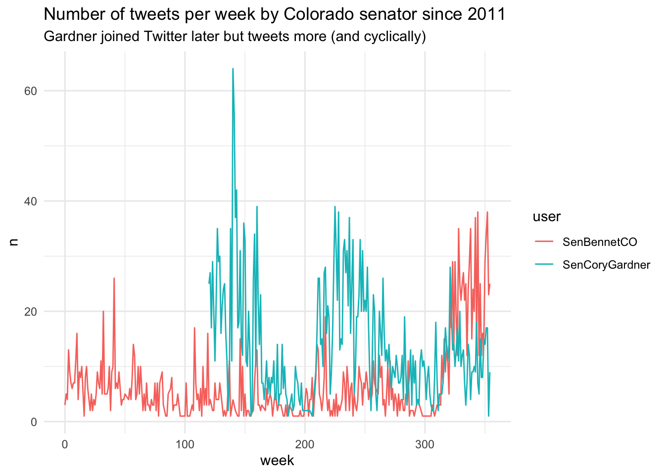
6.6.4 Are tweets correlated in time?
We arbitrarily selected “weekly number of tweets” by each senator and it’s possible that tweet volume in a prior week correlate with tweet volume in a subsequent week (i.e., autocorrelation). This calls for an autocorrelation plot! We’ll create one for Senator Gardner.
# create a data frame with only Gardner's tweets
tweets_gardner <- tweets_co_wk %>%
  filter(user == "SenCoryGardner")

# create a partial autocorrelation plot of tweets by week
pacf(tweets_gardner$n, lag.max = 60)  #go out more than 52 weeks to see annual correlation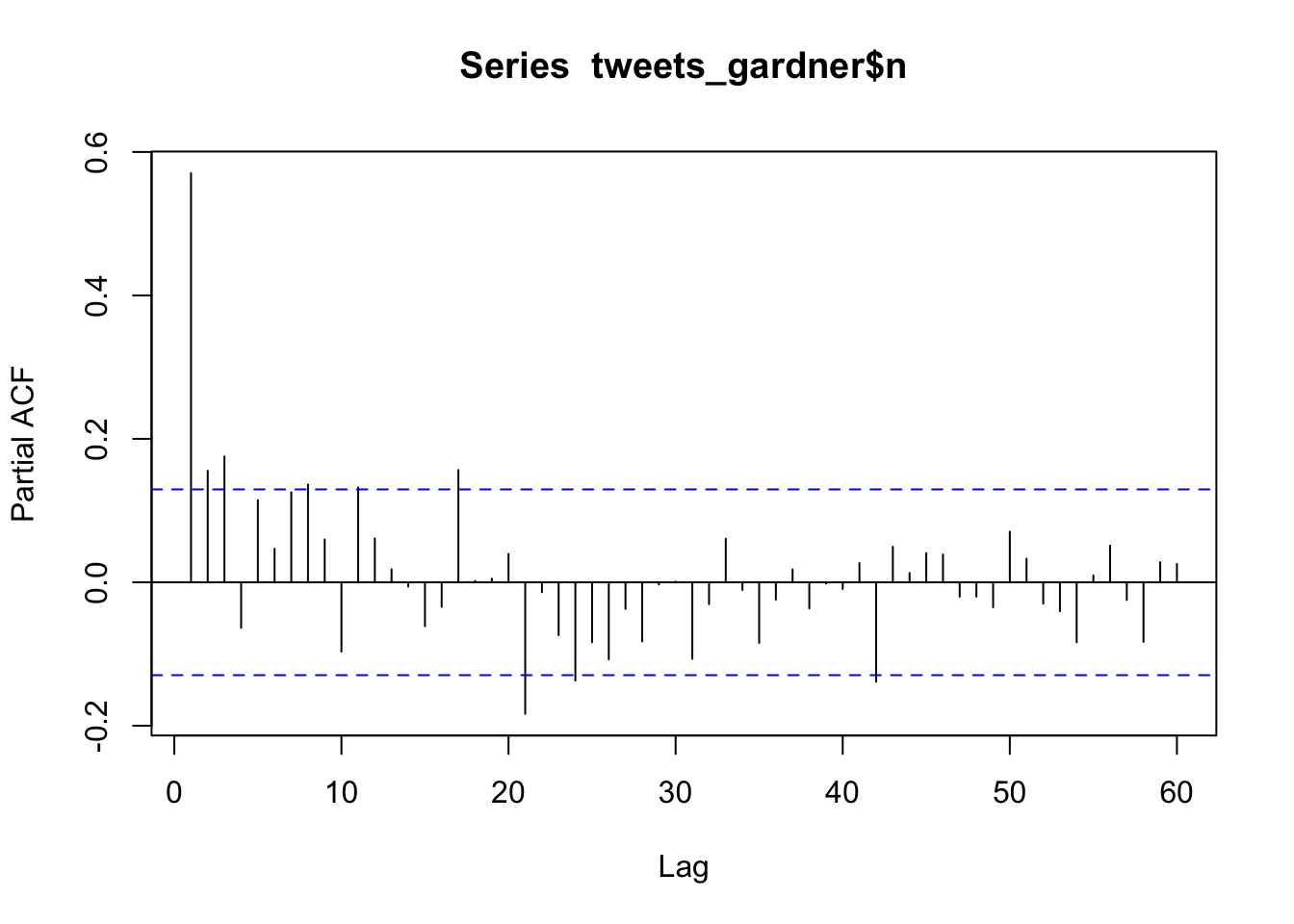
It appears, as one might expect, that tweets are correlated in time. Most of the correlation happens in the first three lags, so maybe these data would be better suited for a monthly average…
6.6.5 Set 4: CSU vs. CU
- How many times are strings related to CSU mentioned by each senator by year?
This might include things like “CSU”, “colostate”, “Colostate”, “Colorado State
U”, “Rams”, etc. You will need to use a few
dplyrfunctions, onelubridatefunction, and onestringrfunction within the pipeline.
# determine number of csu-related tweets by senator per year
tweets_co %>%
  dplyr::group_by(user, lubridate::year(date)) %>%
  dplyr::filter(stringr::str_detect(text, "CSU|colostate|Colostate|Colorado State U|RAMS|Rams|csu")) %>%
  dplyr::tally() %>%
  dplyr::ungroup()
## # A tibble: 10 × 3
## user `lubridate::year(date)` n
## <chr> <dbl> <int>
## 1 SenBennetCO 2011 1
## 2 SenBennetCO 2012 1
## 3 SenBennetCO 2013 1
## 4 SenBennetCO 2014 2
## 5 SenBennetCO 2015 2
## 6 SenBennetCO 2017 1
## 7 SenCoryGardner 2013 4
## 8 SenCoryGardner 2015 5
## 9 SenCoryGardner 2016 2
## 10 SenCoryGardner 2017 2- What is the content of the tweets extracted in the previous question? You
will need to use another
stringrfunction. You can use the same text strings as before.
# extract csu-related tweet content
stringr::str_subset(tweets_co$text,
                    "CSU|colostate|Colostate|Colorado State U|RAMS|Rams|csu")
## [1] "RT @CSUAgSci: .@SenBennetCO & @SenCoryGardner announce $500K @usda grant to @ColoradoStateU to study Farm to School program https://t.co/kb\xe4\xf3_"
## [2] "Best of luck to @CSUMensBball in #NIT first round against South Dakota State! #GoRams"
## [3] "CSU-led study shows risks for CO if we don't tackle climate change. Risks worsen the longer we wait. It's time to act http://t.co/Nlz4pmj8D6"
## [4] "Congrats to @CSUPFootball on tonight's #NCAAD2 championship win! Great game and even better season. #BackthePack"
## [5] "Just wrapped up day 1 of our #COinnovation tour w/ visit to @CSUenergy engines lab. Day 2 in #GrandJunction tomorrow. http://t.co/2Yt5c09Tn3"
## [6] "Here's my #MarchMadness bracket. How do your picks compare? We'll be rooting for you @CUBuffsMBB and @CSUMensBball! https://t.co/4DCdvryOjb"
## [7] "Good luck to @CSUMensBball against Murray State this morning. #MarchMadness #CSUNCAA"
## [8] "Good luck @cubuffs, @CSUFootball and @UNCOFOOTBALL this season. #gobuffs #Rams #BearNation"
## [9] "RT @NewsCPR: .@SenCoryGardner on @CSUPoliSci's John Straayer: \"thanks for being that life-changing spark\"\r https://t.co/LM3CghawTa #copolit\xe4\xf3_"
## [10] "I visited the @CSUEnergy Powerhouse Energy Campus w/ @ColoradoStateU President Franks to learn more about CSU's cut\xe4\xf3_ https://t.co/uTE7M7v7VN"
## [11] "Met with @ColoradoStateU Chancellor Frank & Vice Chancellor Parsons. My staffers who are fellow Rams joined! https://t.co/bF7LArS9Bw"
## [12] "Congrats to @CSUWomensBball on capturing another Mountain West title & being ranked #22 in the country. Go Rams! https://t.co/wawv4CNZLs"
## [13] "Appreciate Coach Bobo & @CSUFootball backing @CoachToCureMD today. Great cause! #TackleDuchenne!"
## [14] "Nothing beats #AgDay at @ColoradoStateU! Always great being with fellow ram handlers at a @CSUFootball game. http://t.co/v32OhG1Kej"
## [15] "@mitchellbyars @RepJaredPolis There is nothing more stylish than a @ColoradoStateU Rams shirt!"
## [16] "Great to be back in Ft Collins at my alma mater @ColoradoStateU. Thanks @CSUTonyFrank for the hospitality, & go Rams http://t.co/zdIcrsgSdL"
## [17] "Great day to be at the @NationalWestern on CSU Day! And thanks to @BoydPolhamus for the introduction! #NWSS2015 http://t.co/fc46YhoUXg"
## [18] "Go @CSUfootball! #CSURams #BringBackTheBoot Win the #BorderWar"
## [19] "@RepMarthaRoby I'm proud to be a #CSURam @CSUFootball"
## [20] "Go @CSUFootball!!!@UA_Athletics: Happy #RollTide Friday! RT if you're ready for @AlabamaFTBL vs. Colorado State! #CSUvsBAMA"
## [21] "#GoRams! #RMShowdown. @CSUfootball: #BeatTheBuffs. -cg"- Which Colorado senator tweets the most about University of Colorado? Use a similar approach to Question 7, with strings related to CU, such as “Buffs” or “University of Colorado”.
# number of cu-related tweets by senator per year
tweets_co %>%
  dplyr::group_by(user, lubridate::year(date)) %>%
  dplyr::filter(year(date) >= 2013) %>%
  dplyr::filter(stringr::str_detect(text,
                                    "CU|Buffs|buffs|University of Colorado")) %>%
  dplyr::tally() %>%
  dplyr::ungroup()
## # A tibble: 9 × 3
## user `lubridate::year(date)` n
## <chr> <dbl> <int>
## 1 SenBennetCO 2013 3
## 2 SenBennetCO 2014 2
## 3 SenBennetCO 2015 3
## 4 SenBennetCO 2016 3
## 5 SenBennetCO 2017 3
## 6 SenCoryGardner 2013 6
## 7 SenCoryGardner 2015 11
## 8 SenCoryGardner 2016 5
## 9 SenCoryGardner 2017 36.7 Chapter 6 Homework
You will continue to use the FiveThirtyEight Twitter data for homework.
Download the csv from Canvas containing Colorado senators’ tweets from 2011 to 2017 (not the full data file used in the above exercises) and the R Markdown template. Your knitted submission is due at the start of the first class of the next chapter.